Visualization for Machine Learning

Spring 2024

Agenda

1. Clustering
2. Dimensionality Reduction

Clustering

Etienne Bernard: “… the goal of clustering is to separate a set of examples into groups called clusters”

IRIS

# Code source: Gaël Varoquaux
# Modified for documentation by Jaques Grobler
# License: BSD 3 clause
#
import matplotlib.pyplot as plt

from sklearn import datasets
iris = datasets.load_iris()

_, ax = plt.subplots()
scatter = ax.scatter(iris.data[:, 2], iris.data[:, 1])
ax.set(xlabel=iris.feature_names[2], ylabel=iris.feature_names[1])
_ = ax.legend(
    scatter.legend_elements()[0], iris.target_names, loc="lower right", title="Classes"
)

IRIS

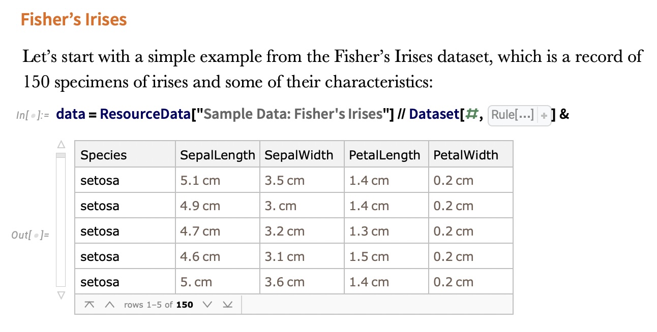
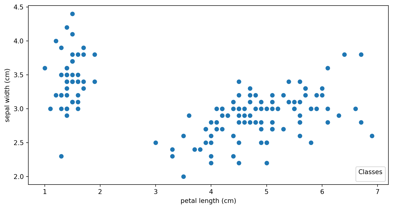
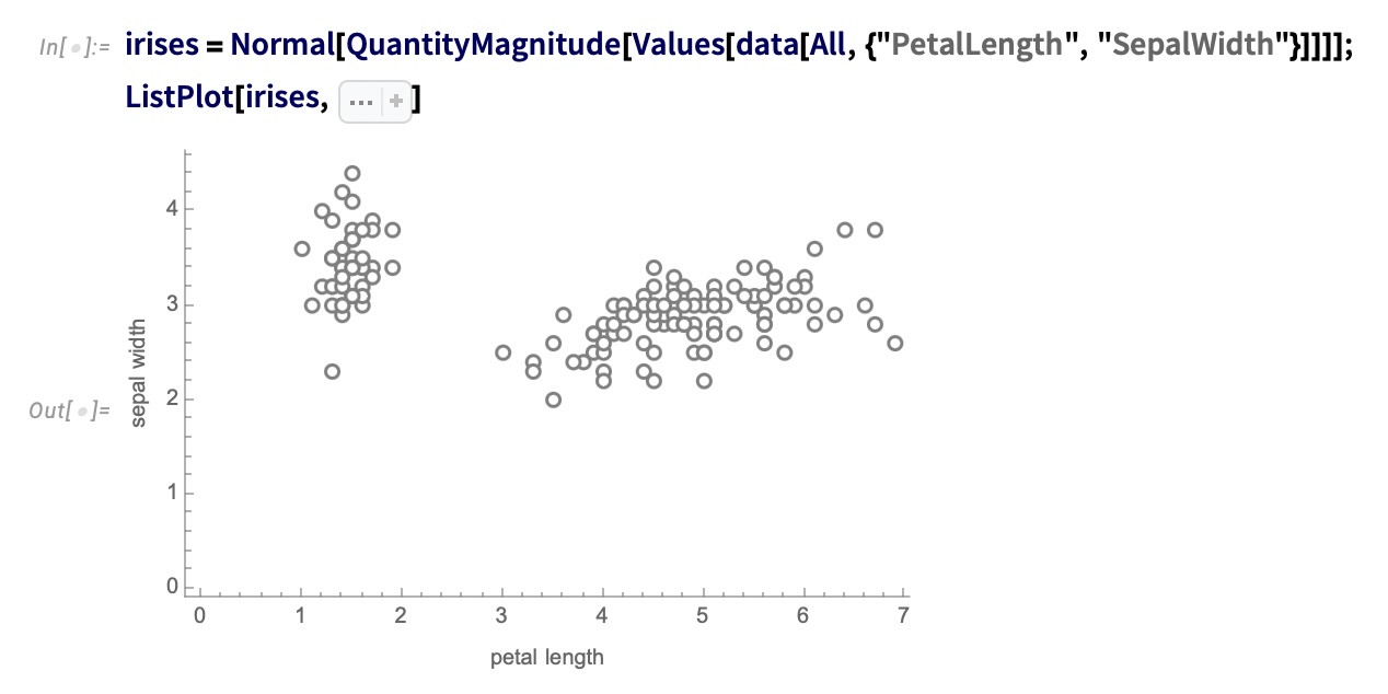
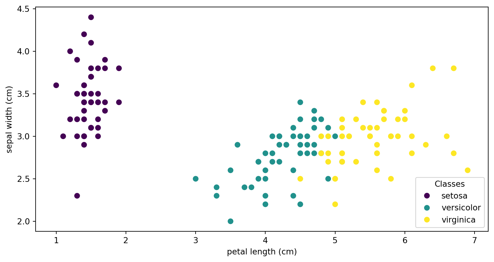
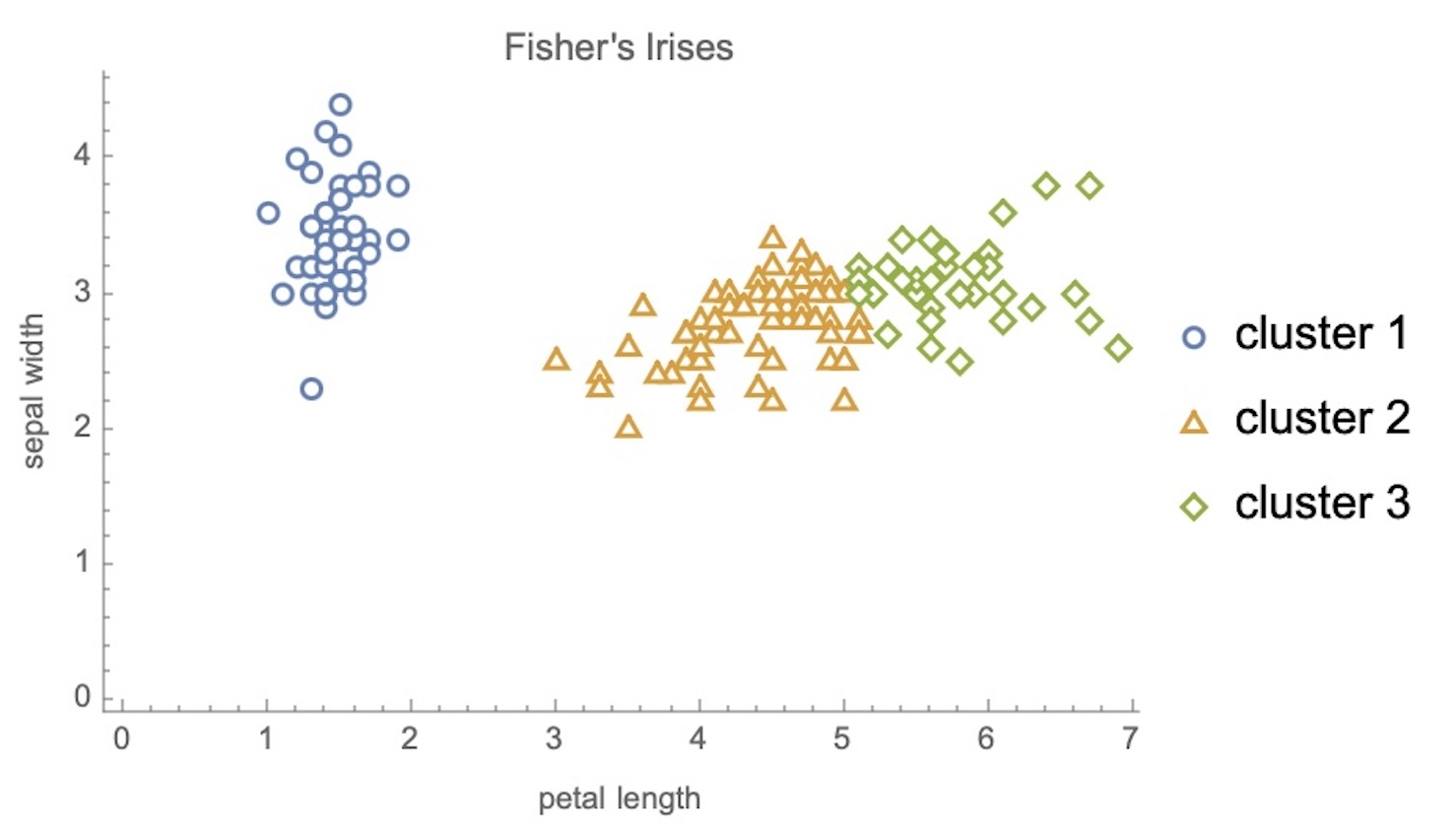
IRIS – another look (Bernard)

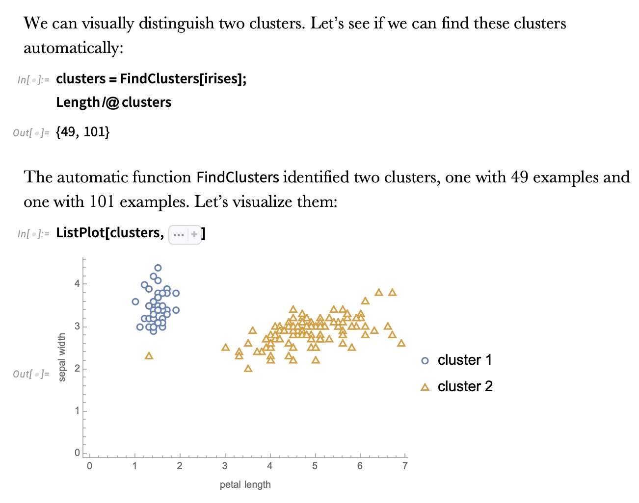
IRIS – clustering

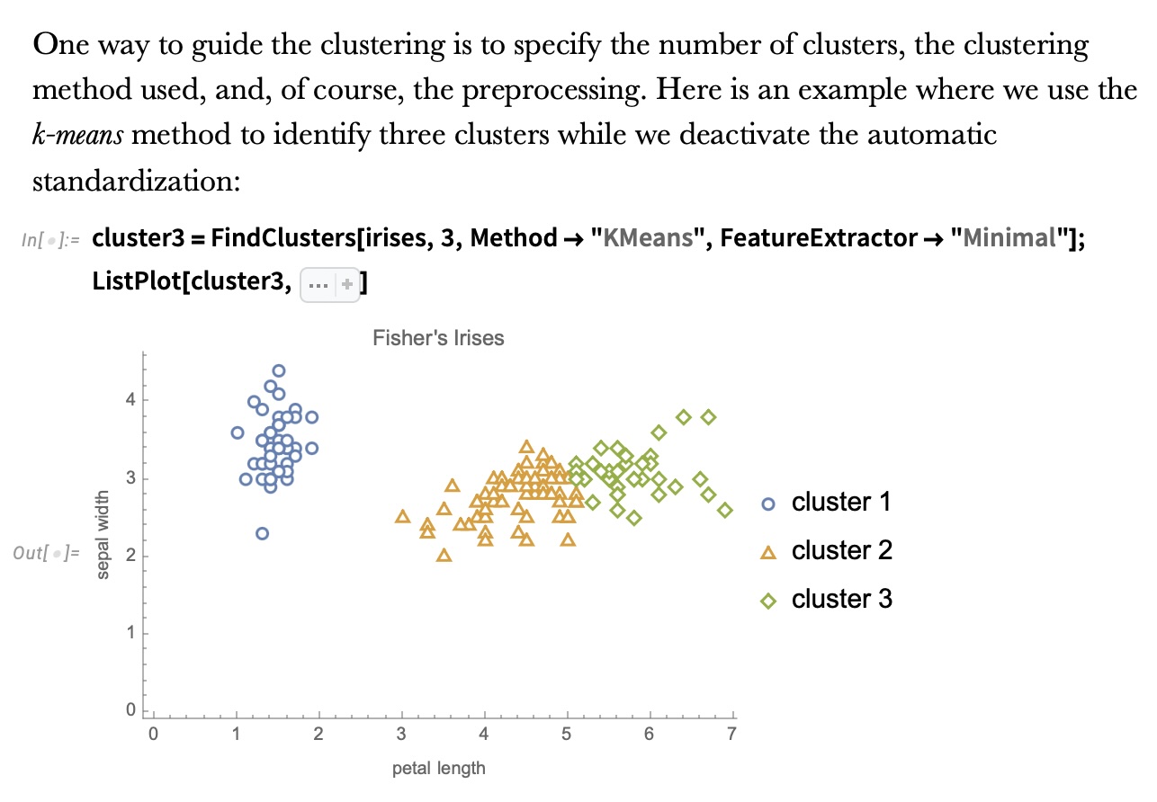
IRIS – k-means

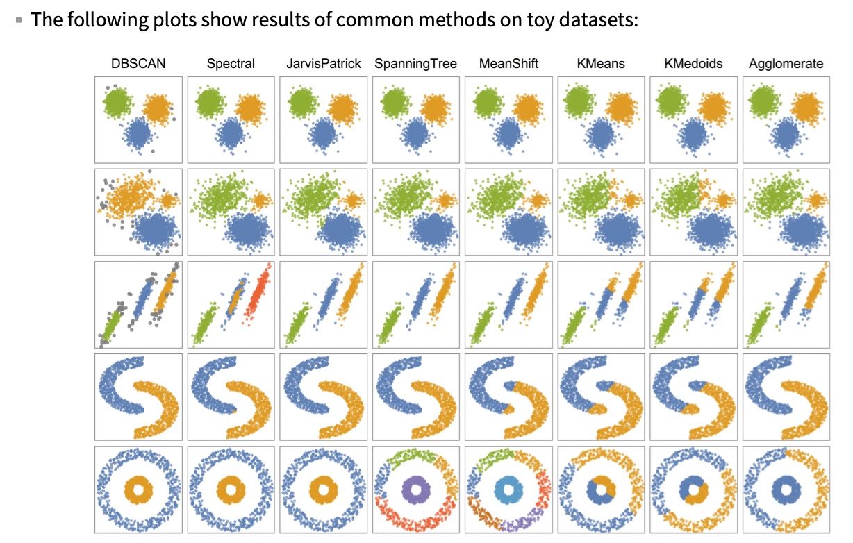
Wolfram Mathematica FindClusters

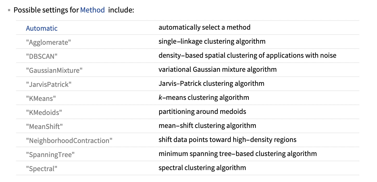
Wolfram Mathematica FindClusters

IRIS - classes

Recommended reading

• Required https://www.wolfram.com/language/introduction-machine-learning/clustering/ link

• https://en.wikipedia.org/wiki/Cluster_analysis

• https://en.wikipedia.org/wiki/K-means_clustering

• https://en.wikipedia.org/wiki/DBSCAN

Dimensionality Reduction

• Input data may have thousands or millions of dimensions!

• Dimensionality Reduction represents data with fewer dimensions

  • easier learning – fewer parameters
  • visualization – show high-dimensional data in 2D or 3D
  • discover “intrinsic dimensionality” of the data

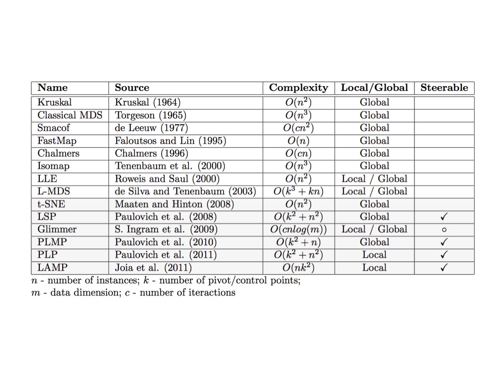
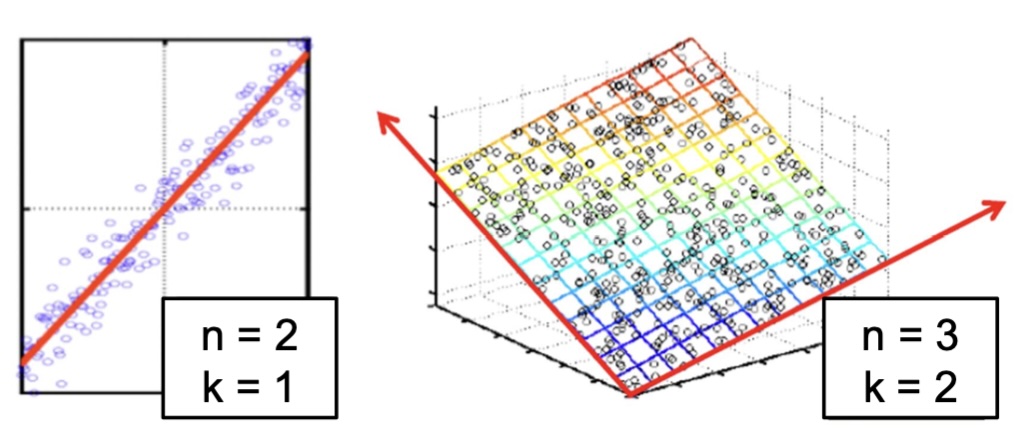
Dimensionality Reduction (Yi Zhang)

• Assumption: data lies on a lower dimensional space

Dimensionality Reduction (Bishop)

• Supposed a dataset of “3s” perturbed in various ways

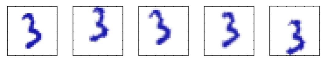
• What operations did we perform? What’s the intrinsic dimensionality?

• Here the underlying manifold is non-linear

Digits

from sklearn.datasets import load_digits

digits = load_digits(n_class=6)
X, y = digits.data, digits.target

Digits - 0

array([[ 0.,  0.,  5., 13.,  9.,  1.,  0.,  0.],
       [ 0.,  0., 13., 15., 10., 15.,  5.,  0.],
       [ 0.,  3., 15.,  2.,  0., 11.,  8.,  0.],
       [ 0.,  4., 12.,  0.,  0.,  8.,  8.,  0.],
       [ 0.,  5.,  8.,  0.,  0.,  9.,  8.,  0.],
       [ 0.,  4., 11.,  0.,  1., 12.,  7.,  0.],
       [ 0.,  2., 14.,  5., 10., 12.,  0.,  0.],
       [ 0.,  0.,  6., 13., 10.,  0.,  0.,  0.]])

Digits - 1

array([[ 0.,  0.,  0., 12., 13.,  5.,  0.,  0.],
       [ 0.,  0.,  0., 11., 16.,  9.,  0.,  0.],
       [ 0.,  0.,  3., 15., 16.,  6.,  0.,  0.],
       [ 0.,  7., 15., 16., 16.,  2.,  0.,  0.],
       [ 0.,  0.,  1., 16., 16.,  3.,  0.,  0.],
       [ 0.,  0.,  1., 16., 16.,  6.,  0.,  0.],
       [ 0.,  0.,  1., 16., 16.,  6.,  0.,  0.],
       [ 0.,  0.,  0., 11., 16., 10.,  0.,  0.]])

Digits

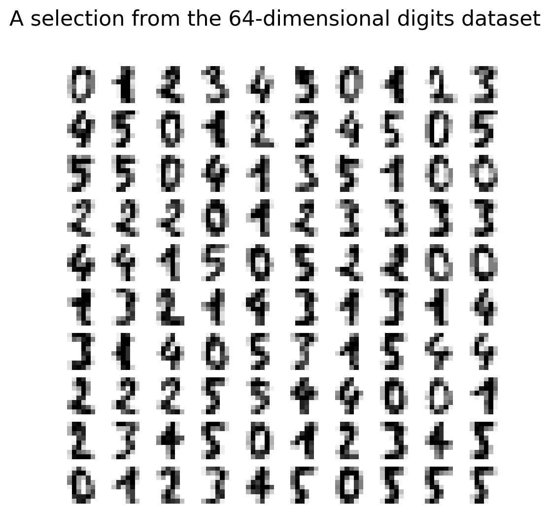
Digits

Computing Random projection embedding...
Computing Truncated SVD embedding...
Computing Linear Discriminant Analysis embedding...
Computing Isomap embedding...
Computing Standard LLE embedding...
Computing Modified LLE embedding...
Computing Hessian LLE embedding...
Computing LTSA LLE embedding...
Computing MDS embedding...
Computing Random Trees embedding...
Computing Spectral embedding...
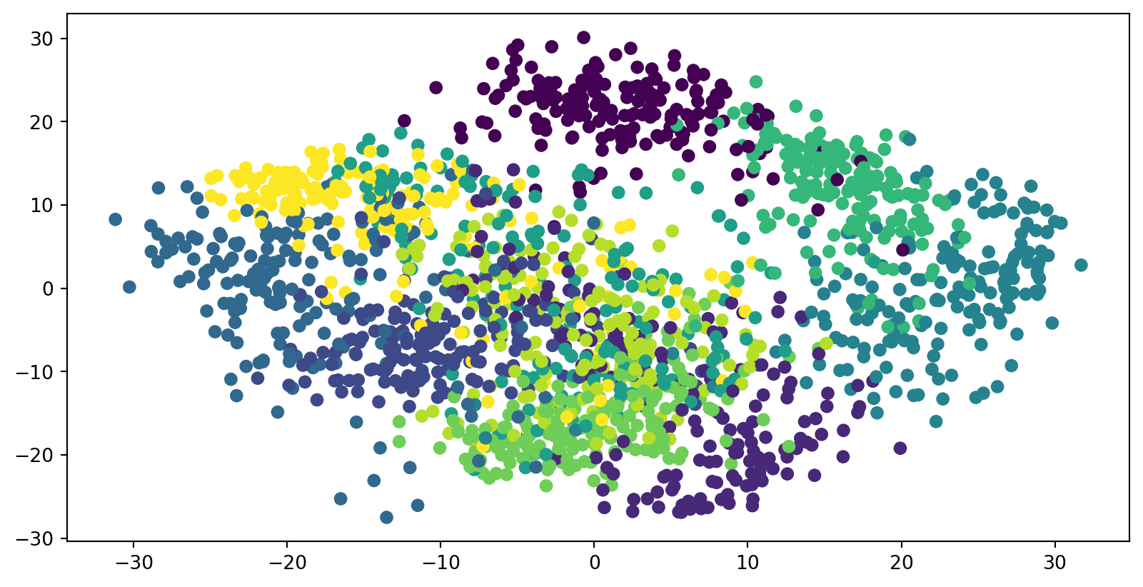
Computing t-SNE embedding...
Computing NCA embedding...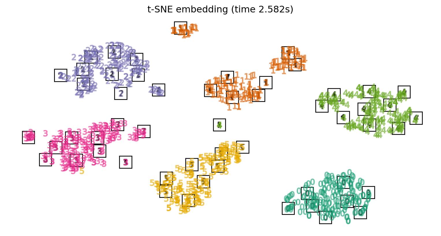

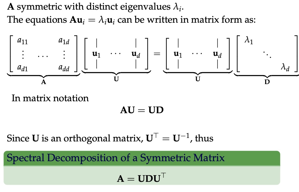
Principal Component Analysis (Luis Gustavo Nonato)

• PCA is directly related to the eigenvectors and eigenvalues of covariance matrices.
• Lets so make a quick review of eigenvectors, eigenvalues, and covariance matrices.

Eigenvectors and Eigenvalues

Given a \(d \times d\) matrix \(A\), a pair \((\lambda, u)\) that satisfies

\(A u = \lambda u\)

is called eigenvalue \(\lambda\) and corresponding eigenvector \(u\) of \(A\).

Symmetric Matrices

• \(\lambda \in \mathbb{R}\) and \(u \in \mathbb{R}^d\) (no complex numbers involved)
• The eigenvectors are orthogonal

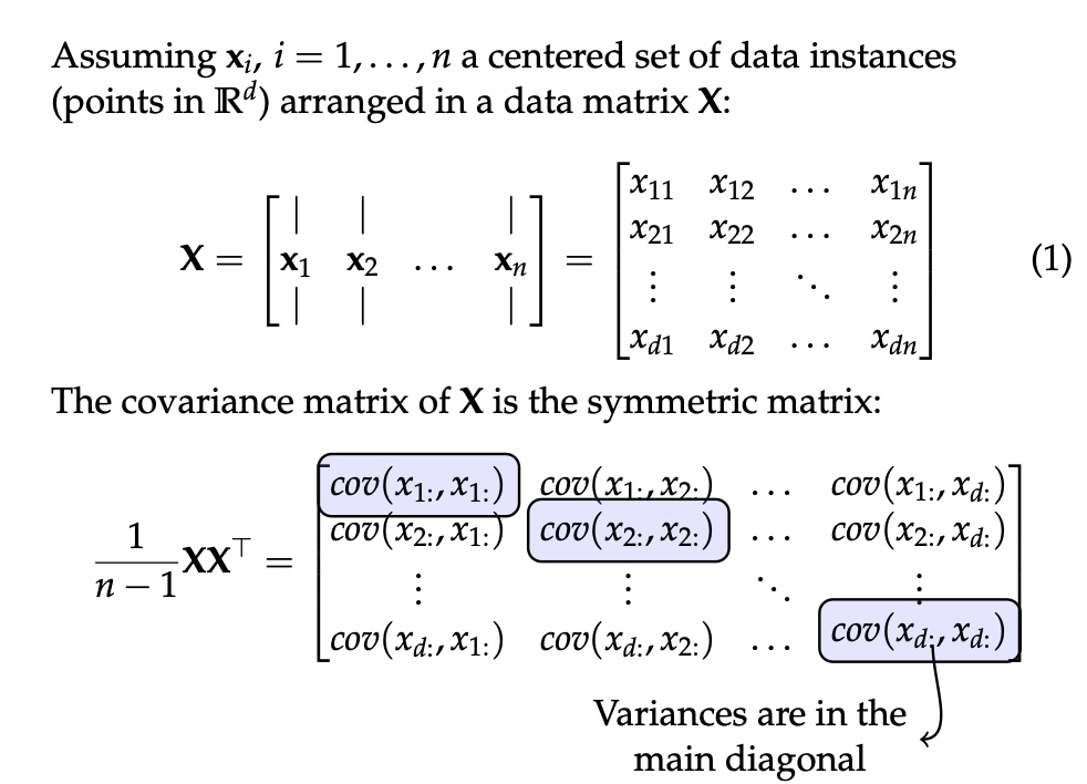
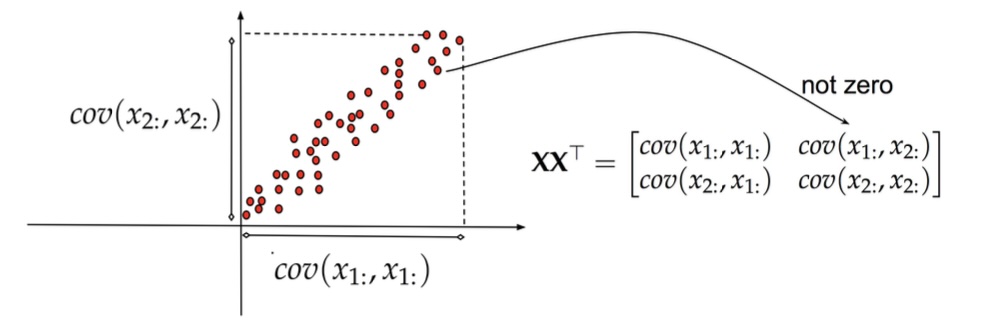
Covariance Matrix

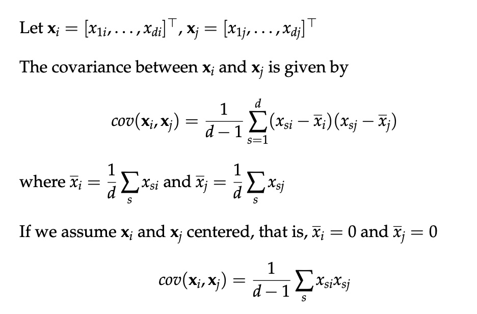
Covariance Matrix

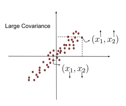
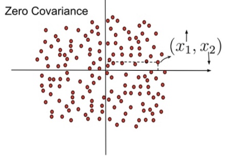
Covariance Matrix

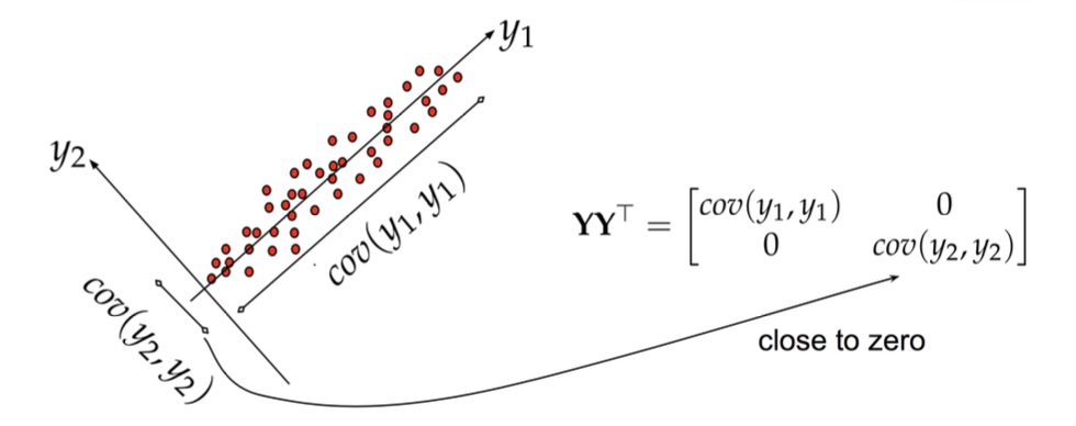
Principal Component Analysis: intuition

Principal Component Analysis: intuition

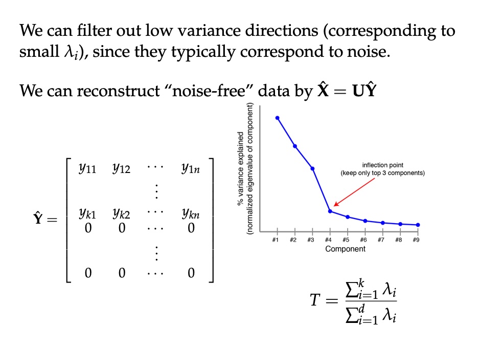
Principal Component Analysis

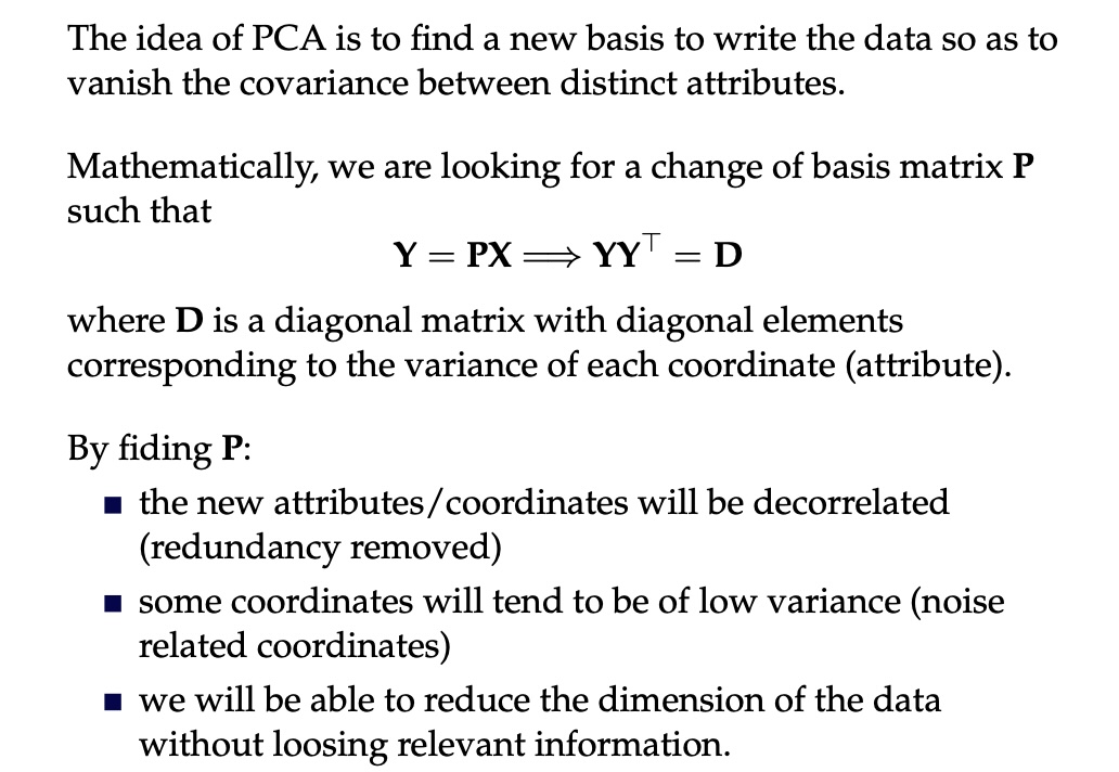
Principal Component Analysis

PCA of digits

PCA of digits

Scaling Up

• Covariance matrix can be really big!
  • \(\Sigma\) is \(n\) by \(n\)
  • 10000 features are not uncommon
  • computing eigenvectors is slow…
• Solution: Singular Value Decomposition (SVD)
  • Finds the \(k\) largest eigenvectors
  • Widely implemented robustly in major packages

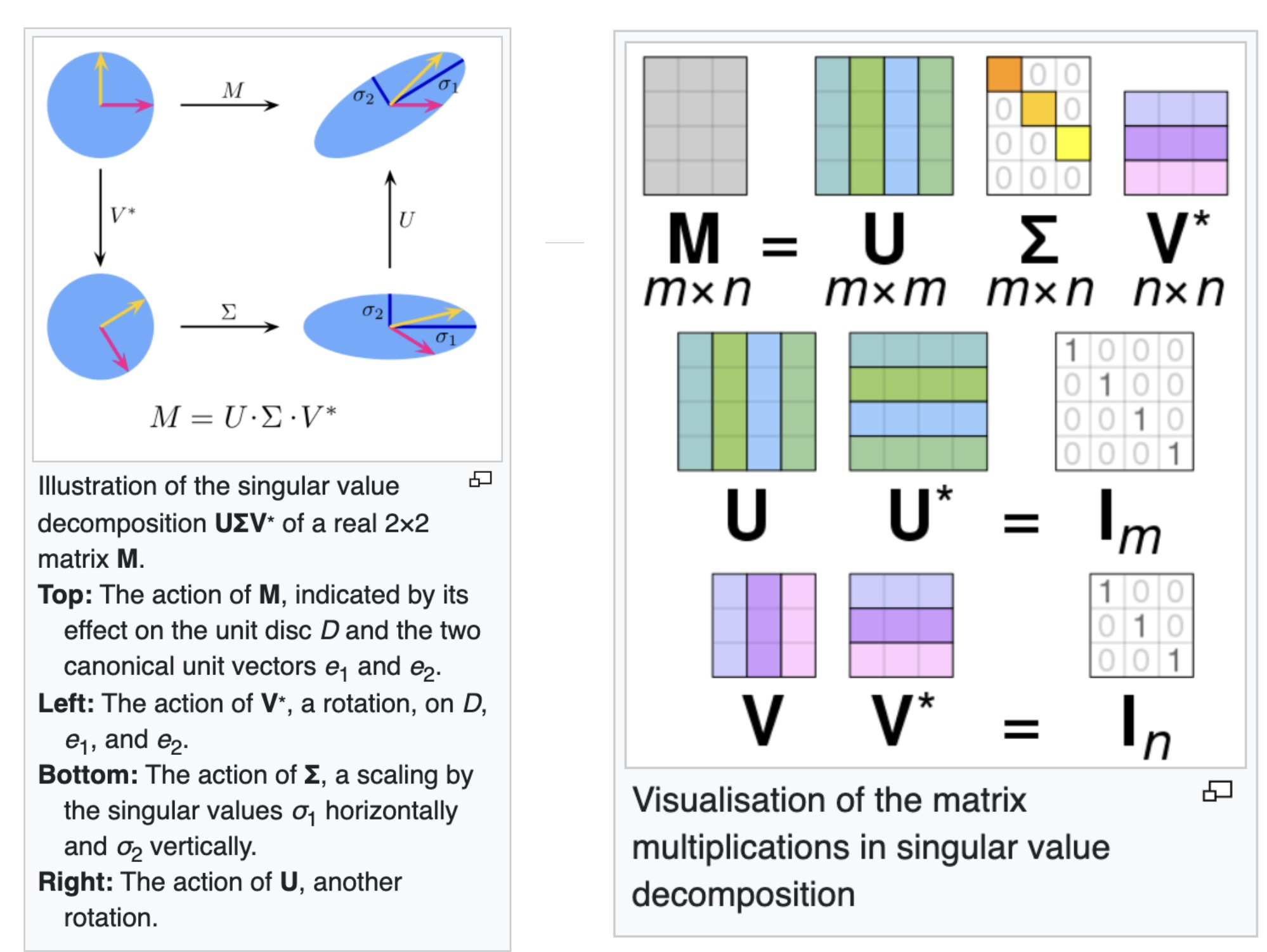
Singular Value Decomposition (SVD)

• https://en.wikipedia.org/wiki/Singular_value_decomposition

Dimensionality Reduction Techniques

• https://en.wikipedia.org/wiki/Dimensionality_reduction
  • Principal component analysis (PCA)
  • Non-negative matrix factorization (NMF)
  • Linear discriminant analysis (LDA)
  • t-SNE
  • UMAP
  • many others

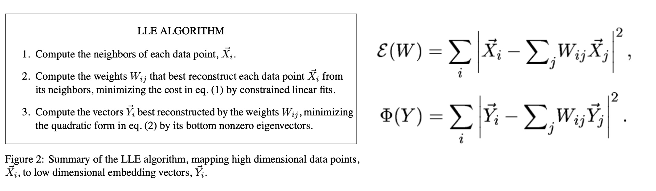
Local Linear Embedding

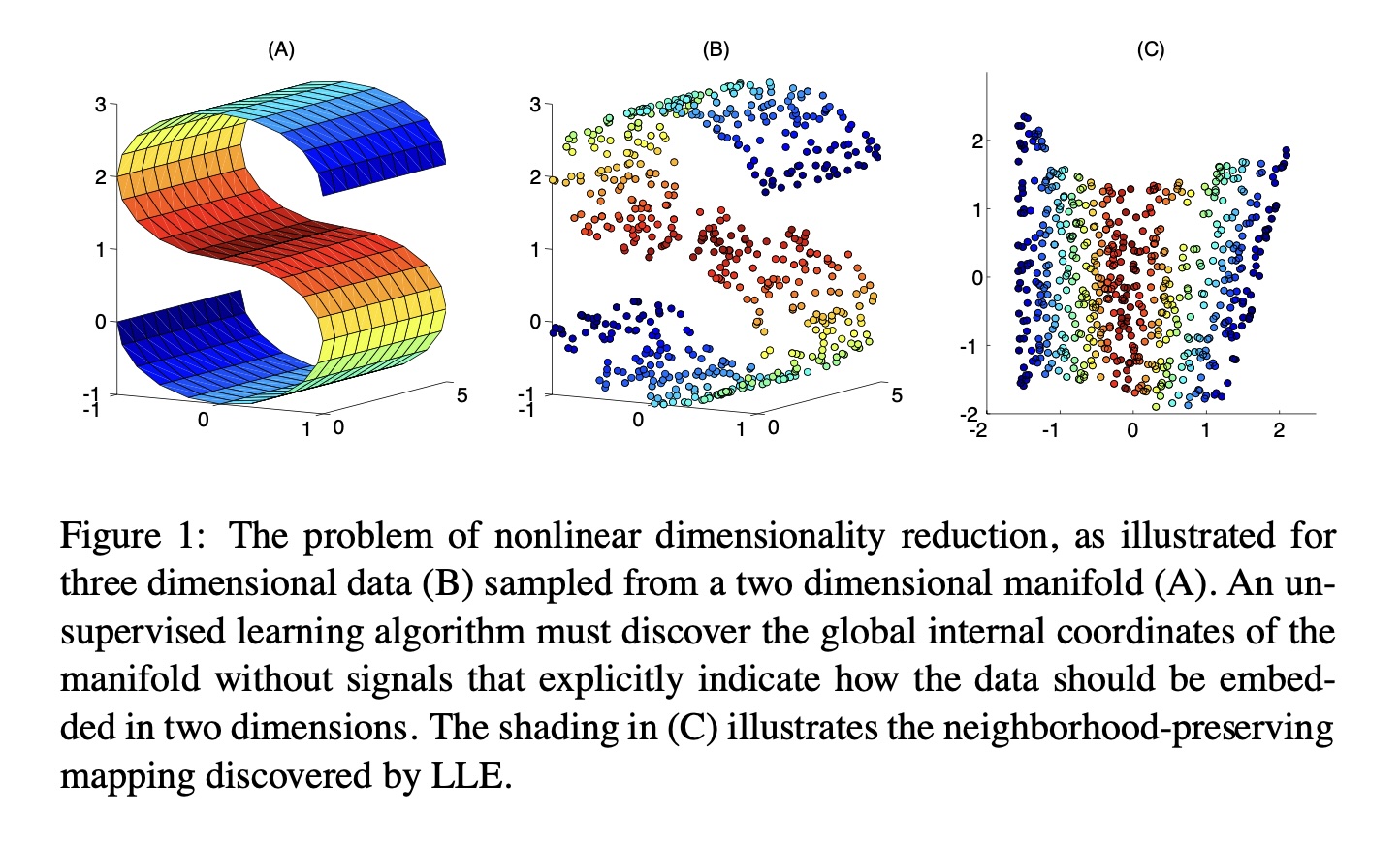
Preserving Local Manifold Neighborhoods

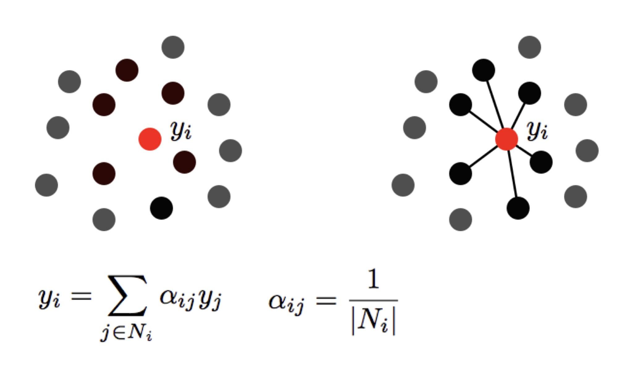
LLE

https://www.science.org/doi/10.1126/science.290.5500.2323

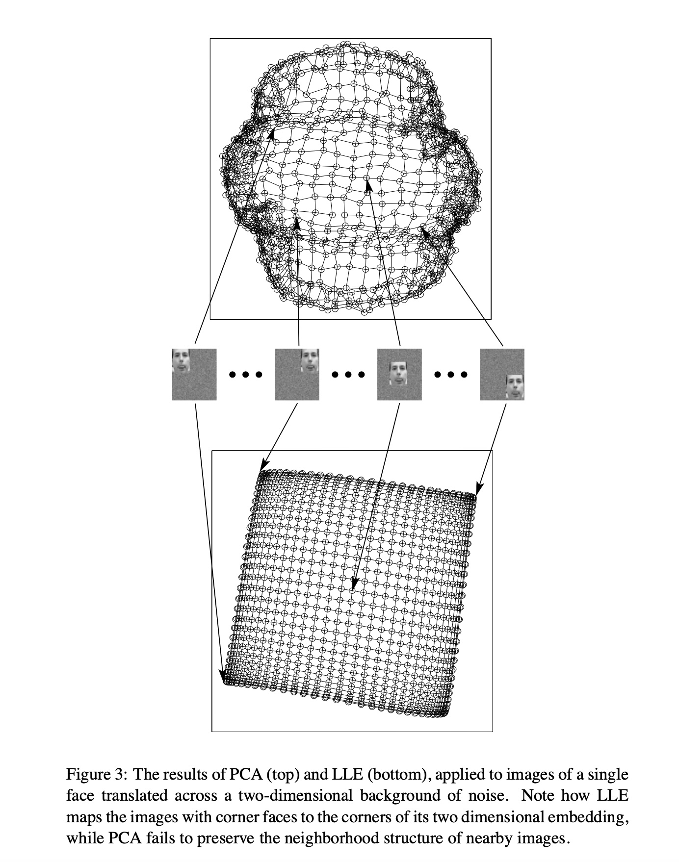
PCA vs LLE

Graph Layout using force based approach

video link

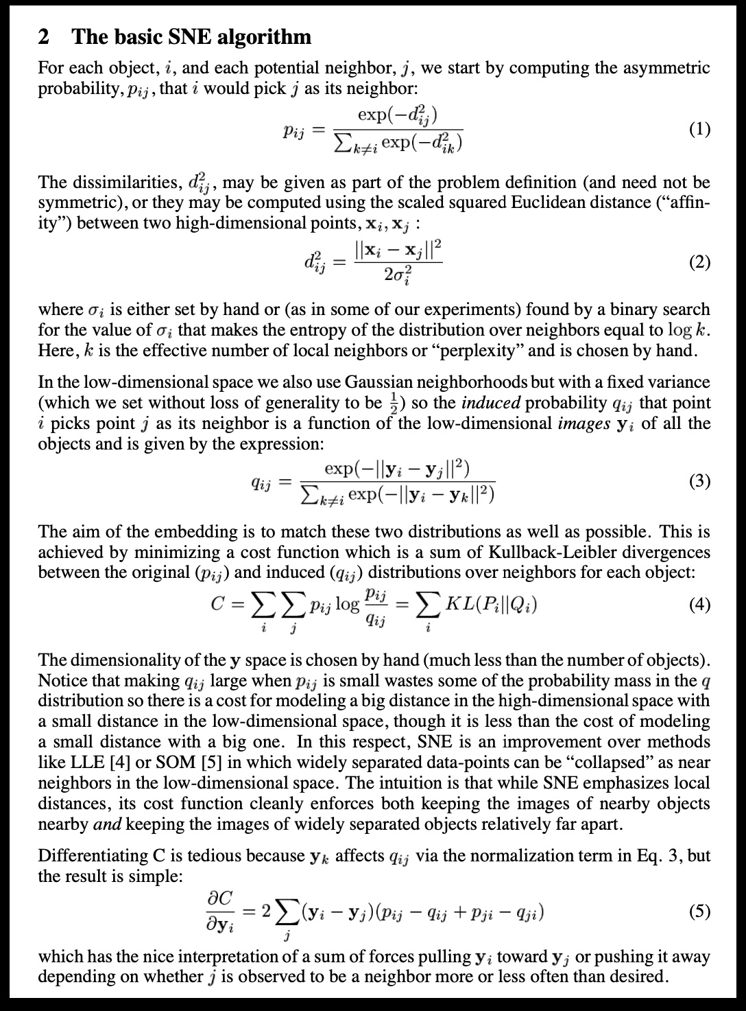
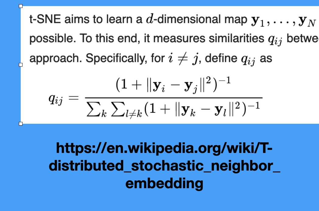
SNE and t-SNE

HERE is an excellent talk by t-SNE creator: video link

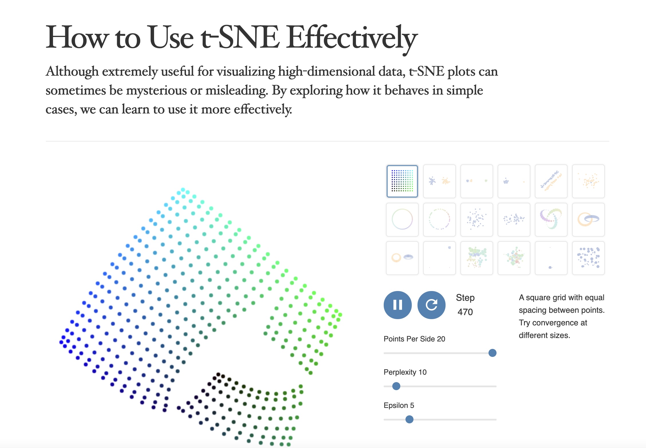
https://distill.pub/2016/misread-tsne/

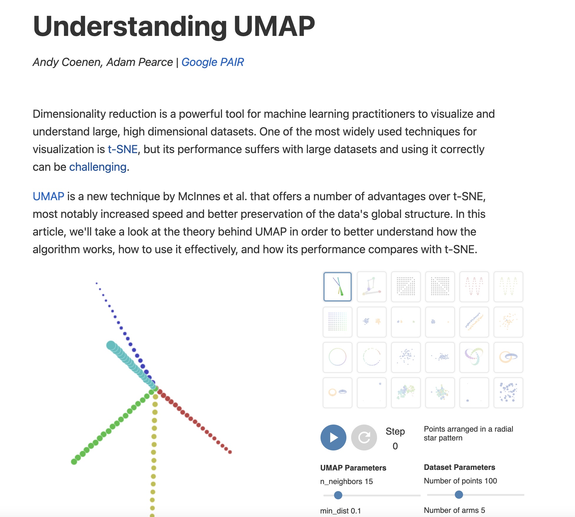
https://pair-code.github.io/understanding-umap/

What about user interaction?