Visualization for Machine Learning

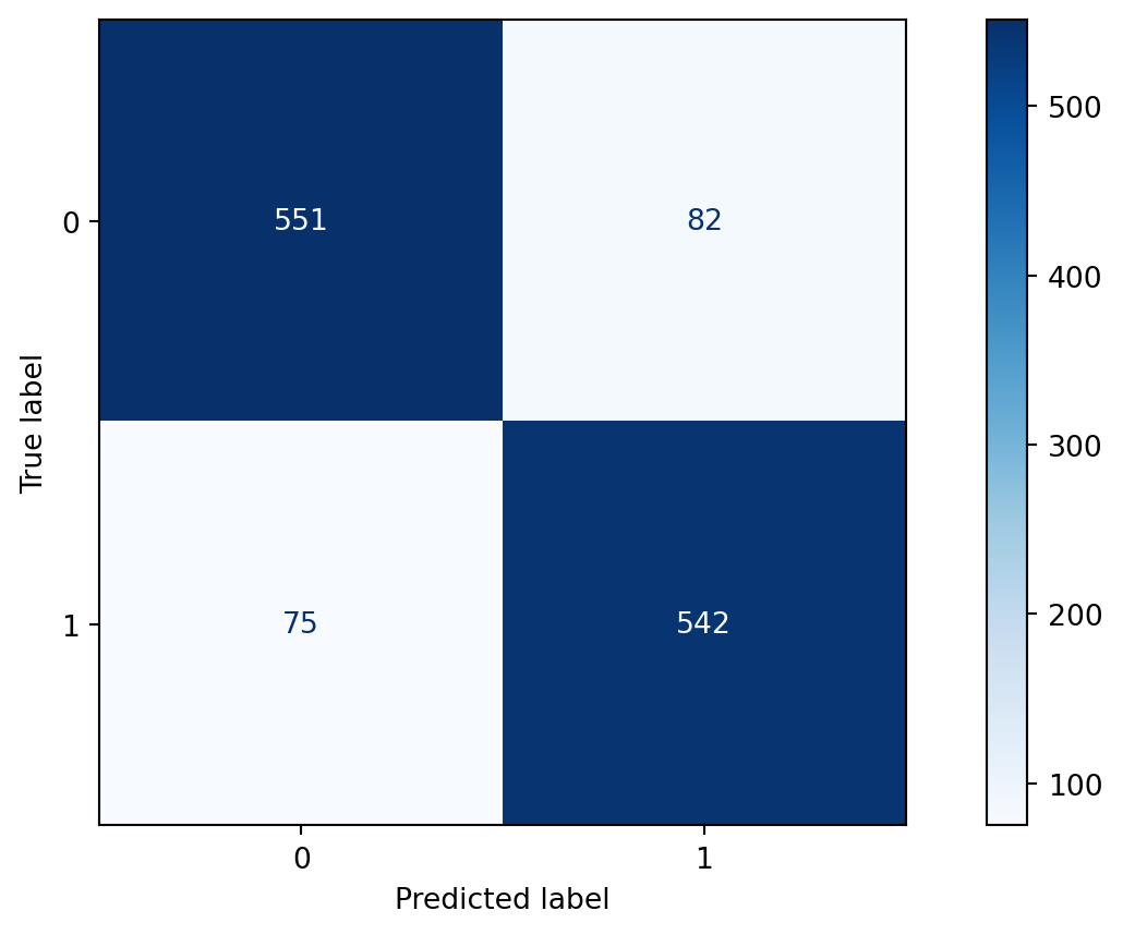
Spring 2024

Model Assessment

Agenda

1. Confusion Matrices and ROC Curves

2. Visual Analytics Systems for Model Performance

3. Calibration

Confusion Matrices, ROC Curves

Scenario: Disease Prediction

• Consider a disease prediction model. Suppose the hypothetical disease has a 5% prevalence in the population

• The given model converges on the solution of predicting that nobody has the disease (i.e., the model predicts “0” for every observation)

• Our model is 95% accurate

• Yet, public health officials are stumped

Scenario: Handwritten Digits

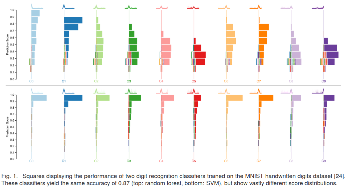
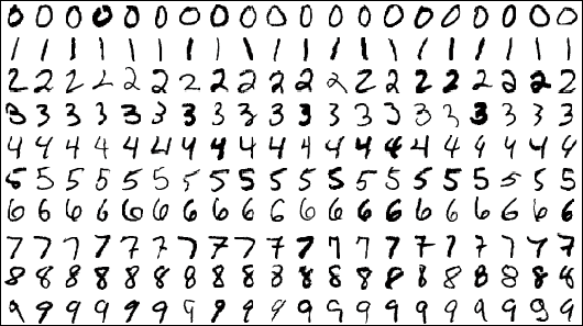
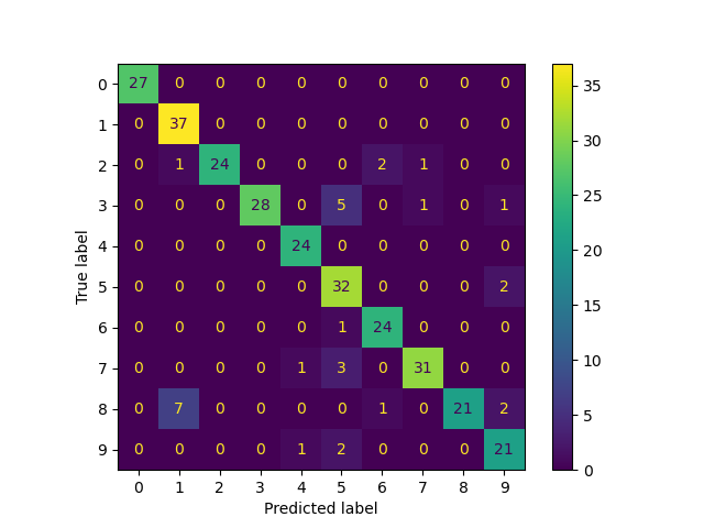
• Consider a model to identify handwritten digits. All digits are equally probable and equally represented in the training and test datasets.

• The model correctly identifies all of the digits, except for digit \(5\), classifying half of the \(5\)s samples as \(6\) and the other half is correctly identified

• The accuracy of this model is \(95\%\). Is this information enough to determine whether the model is good or not?

Extended Confusion Matrix

Confusion Matrices in sklearn

import matplotlib.pyplot as plt
from sklearn.metrics import ConfusionMatrixDisplay

clf.fit(X_train, y_train)

ConfusionMatrixDisplay.from_estimator(clf, X_test, y_test, cmap=plt.cm.Blues)
plt.show()

Confusion Matrices

Pros

• Many derived metrics
  
• Easy to implement
  
• Summary of model mistakes is clear

Cons

• Hard to scale
  
• Hard to assess probabilistic output
  
• Hard to view individual errors

Neo: Hierarchical Confusion Matrix

Receiver Operating Characteristic (ROC)

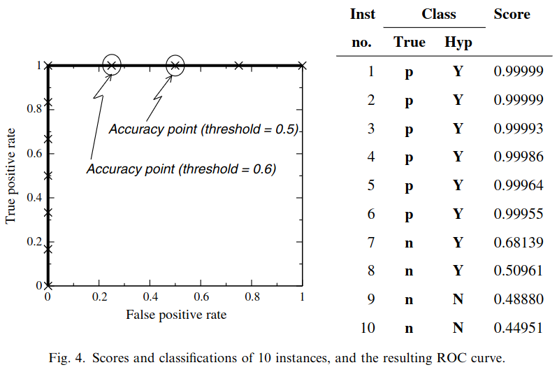
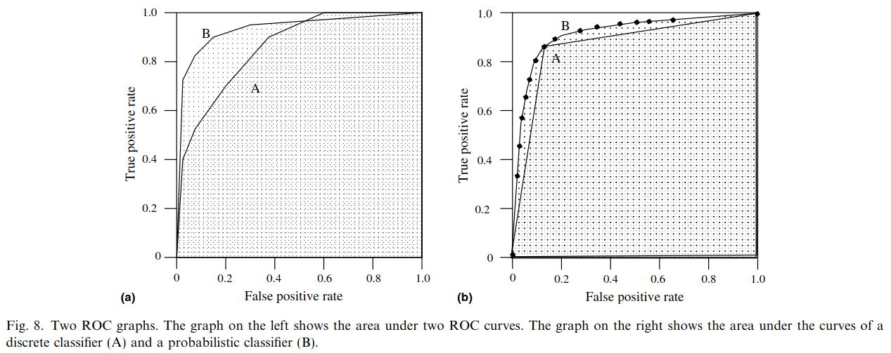
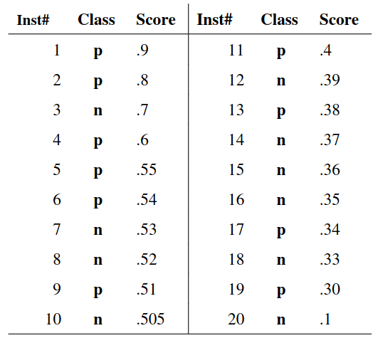
• ROC analysis is another way to assess a classifier’s output

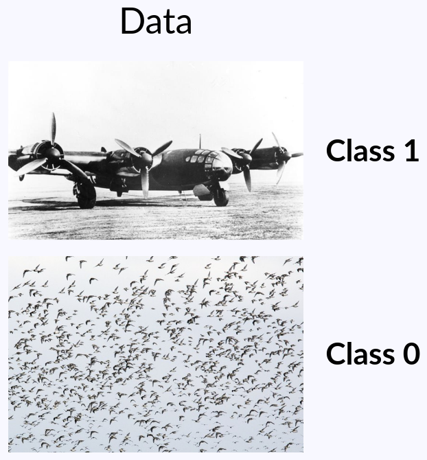
• ROC analysis developed out of radar operation in the second World War, where operators were interested in detecting signal (enemy aircraft) versus noise

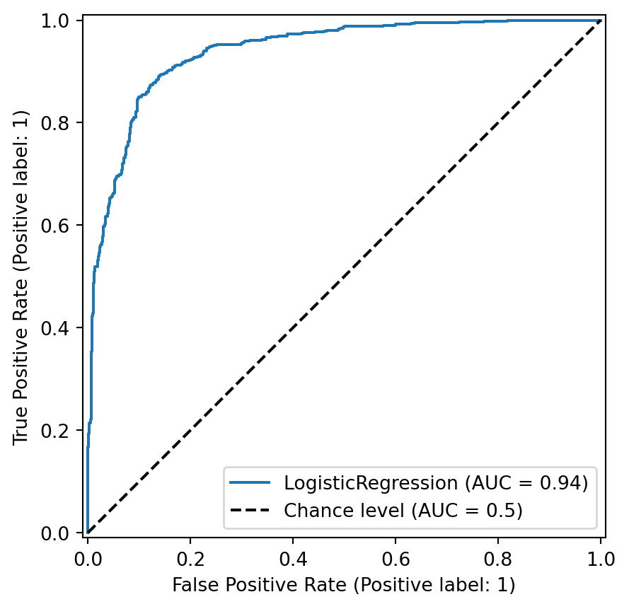
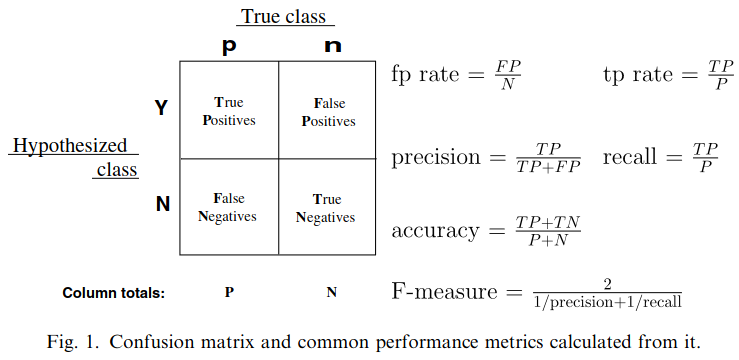
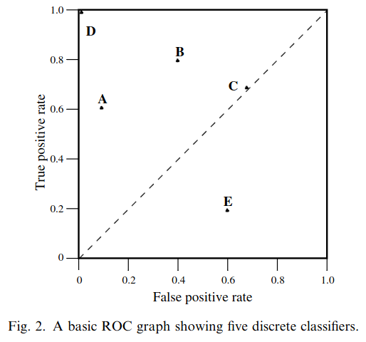
• We create an ROC curve by plotting the true positive rate (TPR) against the false positive rate (FPR) at various thresholds

ROC Curve

ROC Curve

Speaker notes go here.

ROC Curve

Setting the threshold equal to 0.5, we get an accuracy of 80%. However, the curve indicade a perfect classification performance on this test set. Why is there a discrepancy? The model is not properly calibrated. A threshold of 0.7 has perfect accuracy.

Area under an ROC curve (AUC)

ROC curve in sklearn

import matplotlib.pyplot as plt
from sklearn.metrics import RocCurveDisplay

clf.fit(X_train, y_train)

RocCurveDisplay.from_estimator(clf, X_test, y_test, plot_chance_level=True)
plt.show()

Multiclass ROC curve

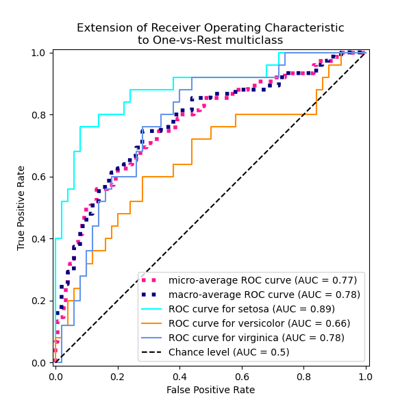
Micro-average: Aggregate contributions of all classes to calculate the metric. Useful if there is class imbalance.

Macro-average: Compute the metric for each class separately, then take average (treats all classes equally)

Visual Analytics Systems for Model Performance

Squares (2016)

Alsallakh et. al. (2014)

Alsallakh et. al. (2014)

Beauxis-Aussalet and Hardman (2014)

Beauxis-Aussalet and Hardman (2014)

EnsembleMatrix (2009)

Calibration

What is calibration?

• When performing classification, we often are interested not only in predicting the class label, but also in the probability of the output

• This probability gives us a kind of confidence score on the prediction

• However, a model can separate the classes well (having a good accuracy/AUC), but be poorly calibrated. In this case, the estimated class probabilities are far from the true class probabilities

• We can calibrate the model, changing the scale of the predicted probabilities

Calibration - Forecast Example

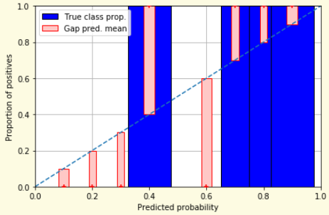
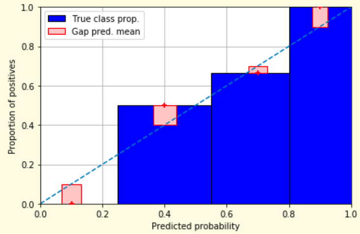
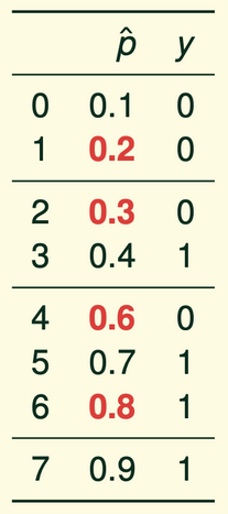
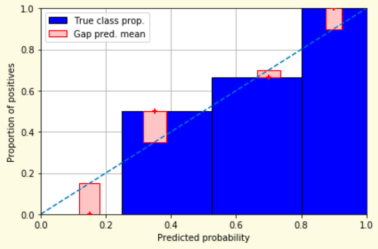
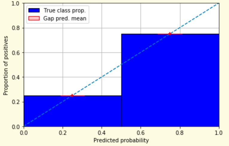
Weather forecasters started thinking about calibration a long time ago (Brier, 1950): a forecast of “70% chance of rain” should be followed by rain 70% of the time. Let’s consider a small toy example:

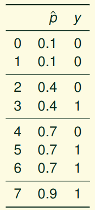
This forecast is doing at predicting the rain:

• “10% chance of rain” was a slight over-estimate: \((\bar{y} = 0/2 = 0\%)\)
• “40% chance of rain” was a slight under-estimate: \((\bar{y} = 1/2 = 50\%)\)
• “70% chance of rain” was a slight over-estimate: \((\bar{y} = 2/3 = 67\%)\)
• “90% chance of rain” was a slight under-estimate: \((\bar{y} = 1/1 = 100\%)\)

Visualizing forecasts - The Reliability Diagram

Reliability diagram - Changing values

Reliability diagram - Changing grouping

Reliability Diagram in sklearn

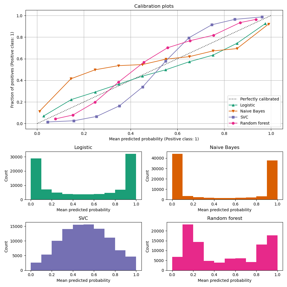
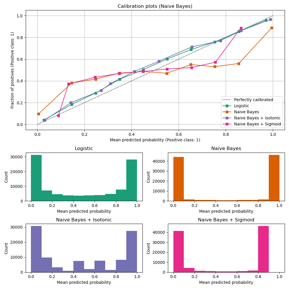
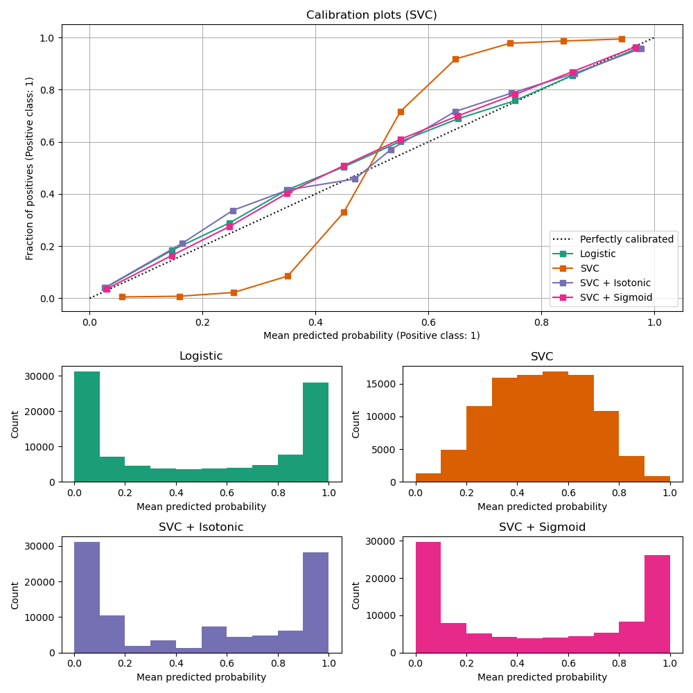
from sklearn.calibration import CalibrationDisplay

fig = plt.figure()
ax = fig.add_subplot(111)

CalibrationDisplay.from_estimator(lg, X_test, y_test, n_bins=10, ax=ax,
                                  label='Logistic Regression')
CalibrationDisplay.from_estimator(nb, X_test, y_test, n_bins=10, ax=ax,
                                  label='Naive Bayes')

<sklearn.calibration.CalibrationDisplay at 0x140862c90>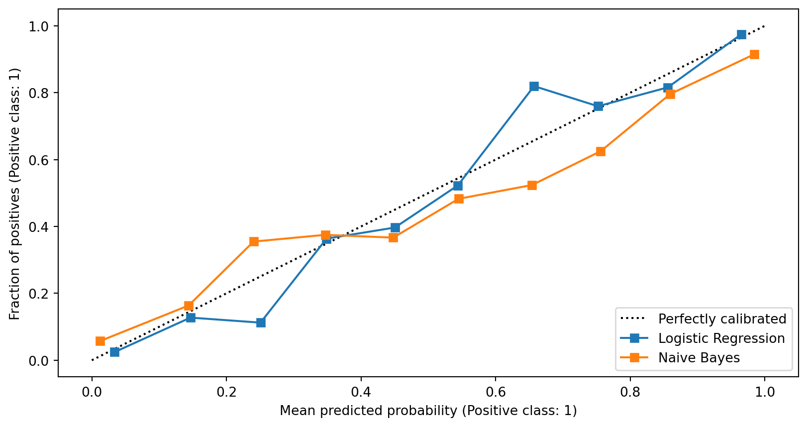

Common sources of miscalibration

• Underconfidence: a classifier thinks it’s worse at separating classes than it actually is.

  • Underconfidence typically gives sigmoidal distortions
  • To calibrate these means to pull predicted probabilities away from the centre

• Overconfidence: a classifier thinks it’s better at separating classes than it actually is

  • Here, distortions are inverse-sigmoidal
  • Calibrating these means to push predicted probabilities toward the centre

A classifier can be overconfident for one class and underconfident for the other

Reliability Diagram in sklearn

Calibration metrics

Let \(N\) be the total of samples, \(B\) the number of binds, \(n^b\) the samples in bin \(b\), and \(conf(b)\) the average predicted probability in bin \(b\).

• Expected Calibration Error:

\[ECE = \sum_{b=1}^B \frac{n^b}{N}|acc(b) - conf(b)|\]

• Maximum Calibration Error:

\[MCE = \underset{m \in \{1,2,\dots,|B|\}}{\text{max}} |acc(b) - conf(b)|\]

Calibration of modern models

Calibration of modern models

Proper Scoring Rules

• Proper scoring rules are calculated at the observation level, where as ECE is binned

• Think of them as putting each item in its separate bin, then computing the average of some loss for each predicted probability and its corresponding observed label

Proper Scoring Rules

• Brier Score/Quadratic error/Euclidean distance:

\[BS = \frac{1}{N} \sum_{i=1}^N (\hat{y}_i - y_i)^2\]

• Log-loss/Cross entropy:

  • Frequently used to as the training loss of machine learning methods, such as neural networks

  • Only penalises the probability given to the true class

\[LL = -\frac{1}{N} \sum_{i=1}^N [y_i \text{log}(\hat{y}_i) + (1-y_i)\text{log}( 1 - \hat{y}_i)]\]

Proper Scoring Rules

An intuitive way to decompose proper scoring rules is into refinement and calibration losses

• Refinement loss: is the loss due to producing the same probability for instances from different classes

• Calibration loss: is the loss due to the difference between the probabilities predicted by the model and the proportion of positives among instances with the same output

Calibration Techniques

Parametric calibration involves modelling the score distributions within each class

• Platt scaling: Logistic calibration can be derived by assuming that the scores within both classes are normally distributed with the same variance (Platt, 2000)

• Beta calibration: employs Beta distributions instead, to deal with scores already on a [0, 1] scale (Kull et al., 2017)

• Dirichlet calibration for more than two classes (Kull et al., 2019)

Non-parametric calibration often ignores scores and employs ranks

• Isotonic regression fits a non-parametric isotonic regressor, which outputs a step-wise non-decreasing function

Platt scaling

• Assumes the calibration curve can be corrected by applying a sigmoid to the raw predictions. This means finding \(\mathbf{A}\) and \(\mathbf{b}\) via MLE:

\[p(y_i = 1 | \hat{y}_i) = \frac{1}{1 + exp(\mathbf{A}\hat{y}_i + \mathbf{b})}\]

• Works best if the calibration error is symmetrical (classifier output for each binary class is normally distributed with the same variance)

• This can be a problem for highly imbalanced classification problems, where outputs do not have equal variance

• In general it is most effective when the un-calibrated model is under-confident and has similar calibration errors for both high and low outputs

Isotonic regression

• Fits a non-parametric isotonic regressor, which outputs a step-wise non-decreasing function

• Isotonic regression is more general when compared to Platt scaling, as the only restriction is that the mapping function is monotonically increasing

• Is more powerful as it can correct any monotonic distortion of the un-calibrated model

• However, it is more prone to overfitting, especially on small datasets

Calibration in sklearn

Calibration in sklearn

Calibration Takeaways

• Reliability diagrams are a standard way to visualize calibration

• ECE is a summary of what reliability diagrams show

• Proper scoring rules (Log loss, Brier score) measure different aspects of probability correctness

• However, proper scoring rules cannot tell us where a model is miscalibrated

Hyperparameters of reliability diagrams

Calibrate (2023)

Calibrate (2023) - Learned Reliability Diagram

Calibrate (2023)

Smooth ECE (2023)

Smooth ECE (2023)

Visualizing Calibration for Multi-Class Problems

Suggested Calibration Literature

• Niculescu-Mizil, A., & Caruana, R. (2005, August). Predicting good probabilities with supervised learning. In Proceedings of the 22nd international conference on Machine learning (pp. 625-632).

• Nixon, J., Dusenberry, M. W., Zhang, L., Jerfel, G., & Tran, D. (2019, June). Measuring Calibration in Deep Learning. In CVPR Workshops (Vol. 2, No. 7).

• Guo, C., Pleiss, G., Sun, Y., & Weinberger, K. Q. (2017, July). On calibration of modern neural networks. In International Conference on Machine Learning (pp. 1321-1330). PMLR.

• Vaicenavicius, J., Widmann, D., Andersson, C., Lindsten, F., Roll, J., & Schön, T. (2019, April). Evaluating model calibration in classification. In The 22nd International Conference on Artificial Intelligence and Statistics (pp. 3459-3467). PMLR.

Suggested Calibration Literature

• Kull, M., & Flach, P. (2015, September). Novel decompositions of proper scoring rules for classification: Score adjustment as precursor to calibration. In Joint European Conference on Machine Learning and Knowledge Discovery in Databases (pp. 68-85). Springer, Cham.

• ECML/PKDD 2020 Tutorial: Evaluation metrics and proper scoring rules

• Google Colab notebook for calibration curves