Visualization for Machine Learning
# Model Assessment ## Agenda \ 1. Confusion Matrices and ROC Curves 2. Visual Analytics Systems for Model Performance 3. Calibration # Confusion Matrices, ROC Curves ## Scenario: Disease Prediction * Consider a disease prediction model. Suppose the hypothetical disease has a 5% prevalence in the population * The given model converges on the solution of predicting that nobody has the disease (i.e., the model predicts “0” for every observation) * Our model is 95% accurate * Yet, public health officials are stumped ## Scenario: Handwritten Digits * Consider a model to identify handwritten digits. All digits are equally probable and equally represented in the training and test datasets. * The model correctly identifies all of the digits, except for digit $5$, classifying half of the $5$s samples as $6$ and the other half is correctly identified * The accuracy of this model is $95\%$. Is this information enough to determine whether the model is good or not? 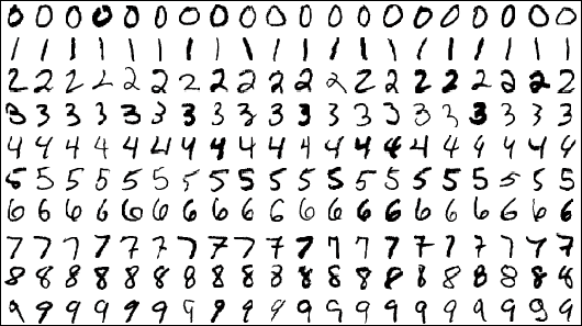{fig-align="center"} ## Extended Confusion Matrix 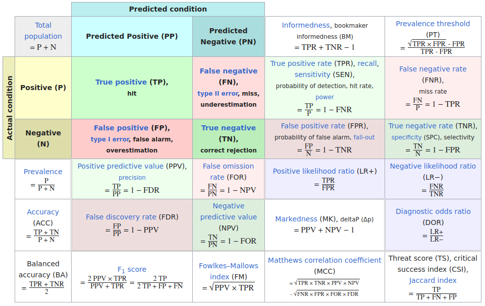{fig-align="center"} ## Confusion Matrices in sklearn ```{python} from sklearn import datasets, svm from sklearn.linear_model import LogisticRegression from sklearn.model_selection import train_test_split X,y = datasets.make_classification(5000, 10, random_state=42) X_train, X_test, y_train, y_test = train_test_split(X, y, random_state=42) clf = LogisticRegression(random_state=0) ``` ```{python} #| echo: true #| fig-pos: c import matplotlib.pyplot as plt from sklearn.metrics import ConfusionMatrixDisplay clf.fit(X_train, y_train) ConfusionMatrixDisplay.from_estimator(clf, X_test, y_test, cmap=plt.cm.Blues) plt.show() ``` ## Confusion Matrices ::::::: {.columns} ::: {.column} 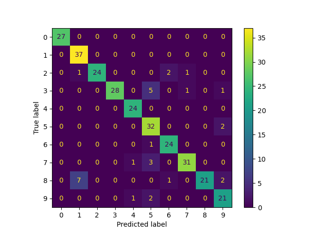 ::: ::: {.column} ::: {.fragment} **Pros** - Many derived metrics\ - Easy to implement\ - Summary of model mistakes is clear ::: ::: {.fragment} **Cons** - Hard to scale\ - Hard to assess probabilistic output\ - Hard to view individual errors ::: ::: :::: ## Neo: Hierarchical Confusion Matrix {fig-align="center"} ## Receiver Operating Characteristic (ROC) :::: {.columns} ::: {.column width="60%"} * ROC analysis is another way to assess a classifier’s output * ROC analysis developed out of radar operation in the second World War, where operators were interested in detecting signal (enemy aircraft) versus noise * We create an ROC curve by plotting the true positive rate (TPR) against the false positive rate (FPR) at various thresholds ::: ::: {.column width="35%"} 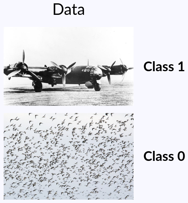 ::: :::: ## ROC Curve :::: {.columns} ::: {.column width="60%"}  ::: {.fragment} 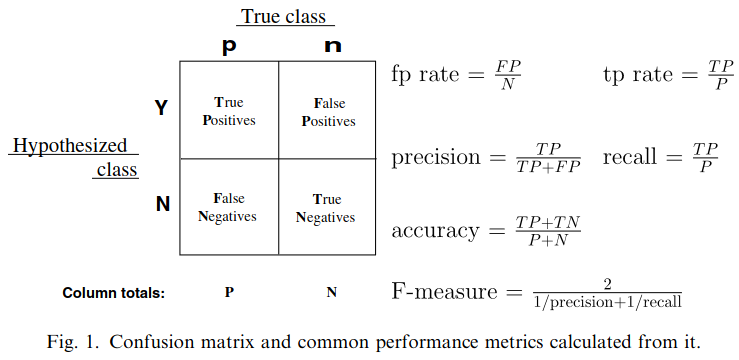 ::: ::: ::: {.column width="40%"} ::: {.fragment} 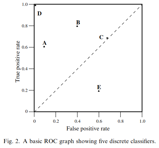 ::: ::: :::: ## ROC Curve :::: {.columns} ::: {.column width="45%"} 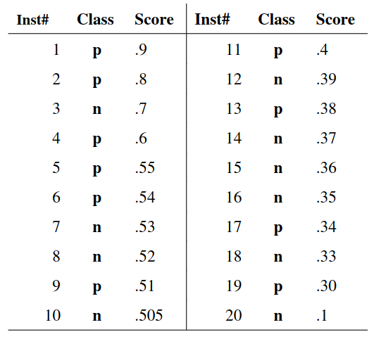 ::: ::: {.column width="55%"}  ::: :::: ::: {.notes} Speaker notes go here. ::: ## ROC Curve 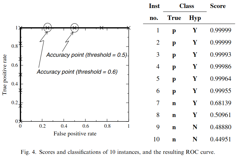{fig-align="center"} ::: {.notes} Setting the threshold equal to 0.5, we get an accuracy of 80%. However, the curve indicade a perfect classification performance on this test set. Why is there a discrepancy? The model is not properly calibrated. A threshold of 0.7 has perfect accuracy. ::: ## Area under an ROC curve (AUC) \ 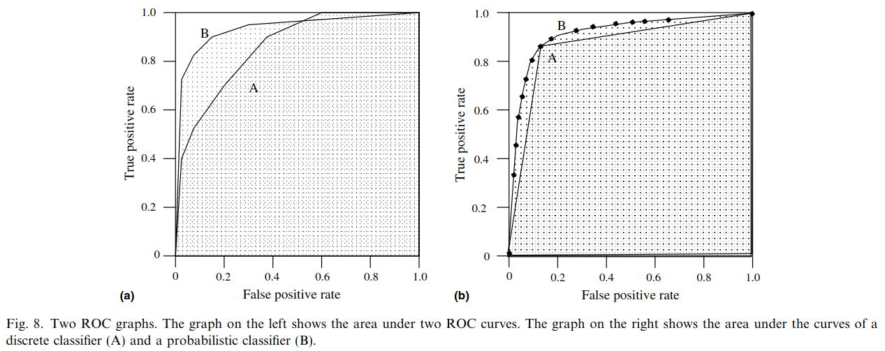{fig-align="center"} ## ROC curve in sklearn ```{python} #| echo: true import matplotlib.pyplot as plt from sklearn.metrics import RocCurveDisplay clf.fit(X_train, y_train) RocCurveDisplay.from_estimator(clf, X_test, y_test, plot_chance_level=True) plt.show() ``` ## Multiclass ROC curve :::: {.columns} ::: {.column width="65%"} 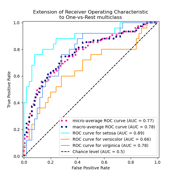{fig-align="center" height=100%} ::: ::: {.column width="35%"} \ **Micro-average:** Aggregate contributions of all classes to calculate the metric. Useful if there is class imbalance. **Macro-average:** Compute the metric for each class separately, then take average (treats all classes equally) ::: :::: :::footer [code](https://scikit-learn.org/stable/auto_examples/model_selection/plot_roc.html) ::: # Visual Analytics Systems for Model Performance ## Squares (2016) 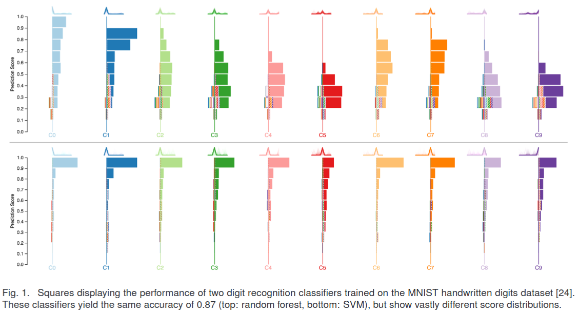{fig-align="center"} :::footer Ren, D., Amershi, S., Lee, B., Suh, J., & Williams, J. D. (2016). *Squares: Supporting interactive performance analysis for multiclass classifiers*. IEEE transactions on visualization and computer graphics. ::: --- ## Alsallakh et. al. (2014) 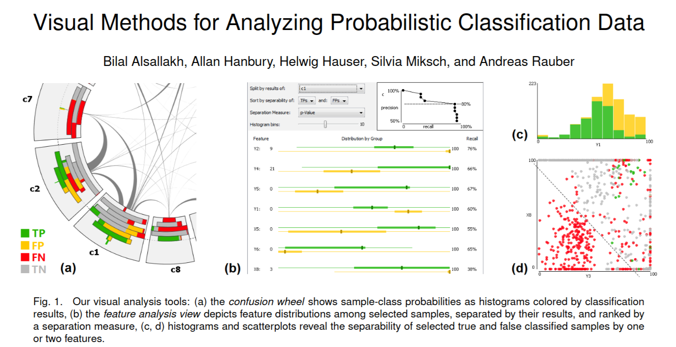{fig-align="center"} :::footer Alsallakh, B., Hanbury, A., Hauser, H., Miksch, S., & Rauber, A. (2014). *Visual methods for analyzing probabilistic classification data*. IEEE transactions on visualization and computer graphics. ::: ## Alsallakh et. al. (2014) 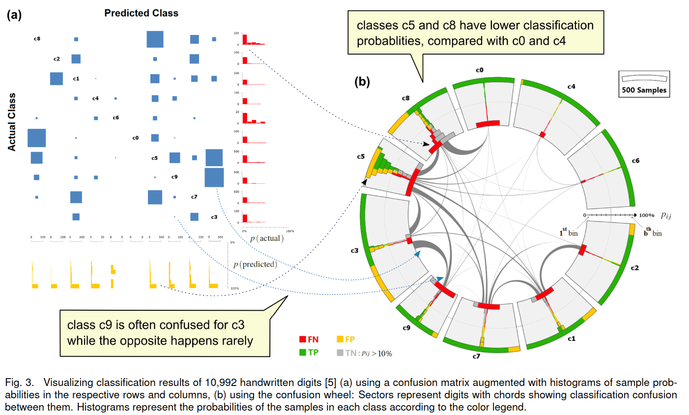{fig-align="center"} :::footer Alsallakh, B., Hanbury, A., Hauser, H., Miksch, S., & Rauber, A. (2014). *Visual methods for analyzing probabilistic classification data*. IEEE transactions on visualization and computer graphics. ::: ## Beauxis-Aussalet and Hardman (2014) \ \ 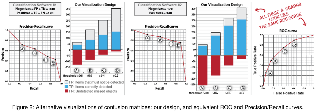{fig-align="center"} :::footer Beauxis-Aussalet, E., & Hardman, L. (2014). *Visualization of confusion matrix for non-expert users*. In IEEE Conference on Visual Analytics Science and Technology (VAST)-Poster Proceedings. ::: ## Beauxis-Aussalet and Hardman (2014) 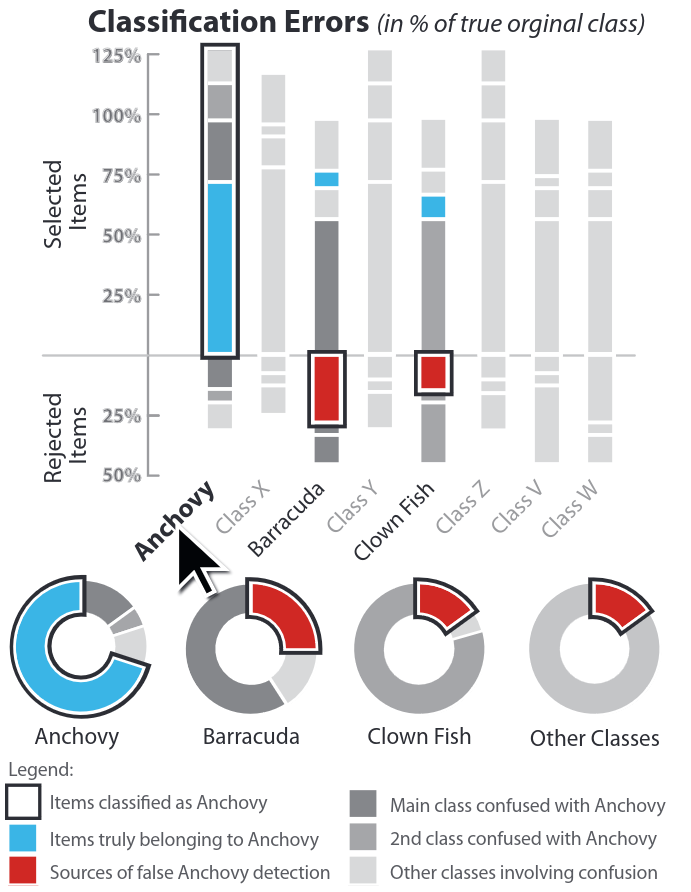{fig-align="center"} :::footer Beauxis-Aussalet, E., & Hardman, L. (2014). *Visualization of confusion matrix for non-expert users*. In IEEE Conference on Visual Analytics Science and Technology (VAST)-Poster Proceedings. ::: ## EnsembleMatrix (2009) 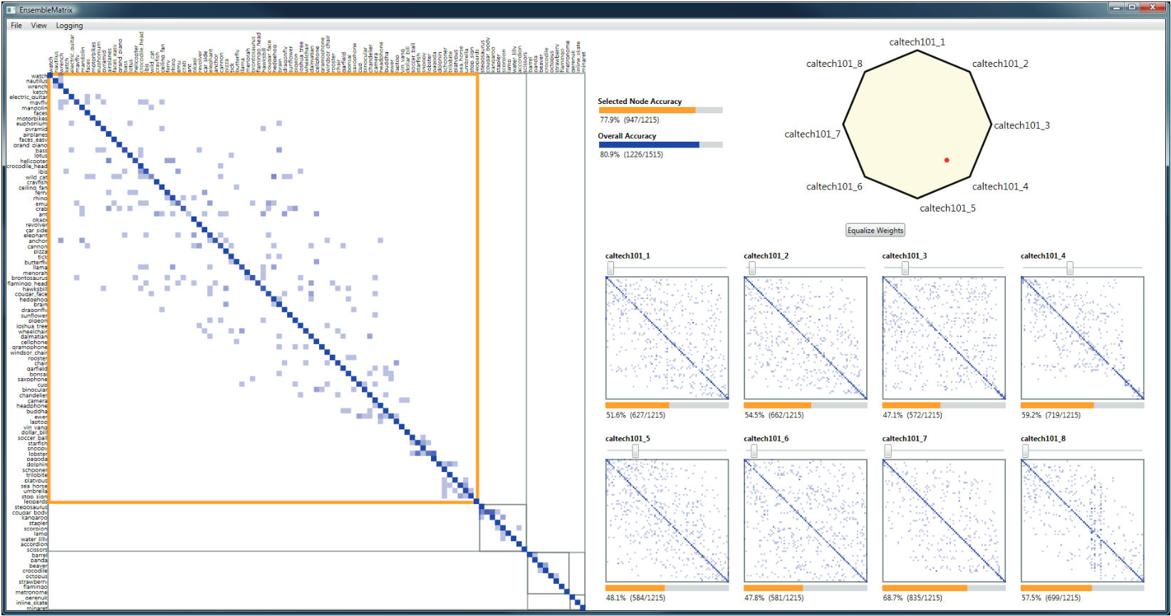{fig-align="center"} :::footer Talbot, J., Lee, B., Kapoor, A., & Tan, D. S. (2009, April). *EnsembleMatrix: interactive visualization to support machine learning with multiple classifiers*. In Proceedings of the SIGCHI conference on human factors in computing systems. ::: # Calibration ## What is calibration? * When performing classification, we often are interested not only in predicting the class label, but also in the probability of the output * This probability gives us a kind of confidence score on the prediction * However, a model can separate the classes well (having a good accuracy/AUC), but be poorly **calibrated**. In this case, the estimated class probabilities are far from the true class probabilities * We can calibrate the model, changing the scale of the predicted probabilities ## Calibration - Forecast Example Weather forecasters started thinking about calibration a long time ago (Brier, 1950): a forecast of "70% chance of rain" should be followed by rain 70% of the time. Let’s consider a small toy example: :::: {.columns} ::: {.column width="30%"} 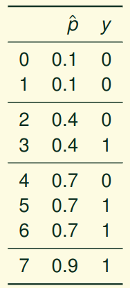{fig-align="center"} ::: ::: {.column width="70%"} This forecast is doing at predicting the rain: - "10% chance of rain" was a slight over-estimate: $(\bar{y} = 0/2 = 0\%)$ - "40% chance of rain" was a slight under-estimate: $(\bar{y} = 1/2 = 50\%)$ - "70% chance of rain" was a slight over-estimate: $(\bar{y} = 2/3 = 67\%)$ - "90% chance of rain" was a slight under-estimate: $(\bar{y} = 1/1 = 100\%)$ ::: :::: ::: footer Slides based on [classifier-calibration.github.io](https://classifier-calibration.github.io/) ::: ## Visualizing forecasts - The Reliability Diagram \ :::: {.columns} ::: {.column width="30%"} {fig-align="center"} ::: ::: {.column width="70%"} 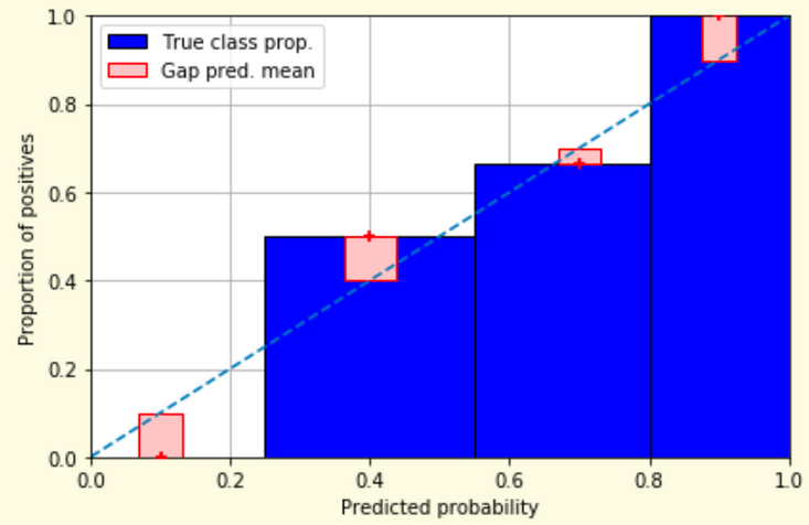{fig-align="center"} ::: :::: ::: footer Slides based on [classifier-calibration.github.io](https://classifier-calibration.github.io/) ::: ## Reliability diagram - Changing values \ :::: {.columns} ::: {.column width="30%"} 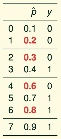{fig-align="center"} ::: ::: {.column width="70%"} 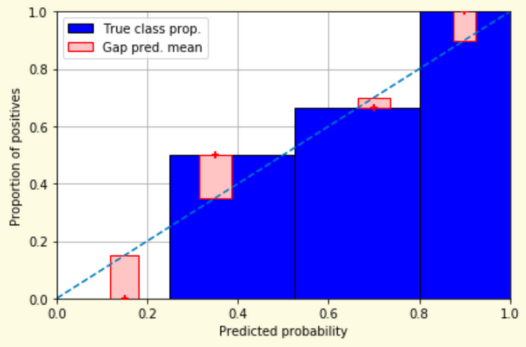{fig-align="center"} ::: :::: ::: footer Slides based on [classifier-calibration.github.io](https://classifier-calibration.github.io/) ::: ## Reliability diagram - Changing grouping \ :::: {.columns} ::: {.column width="30%"} {fig-align="center"} ::: ::: {.column width="70%"} 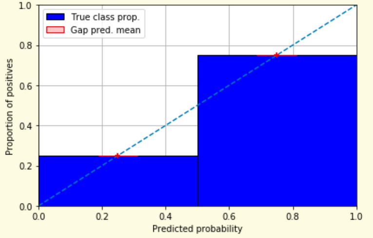{fig-align="center"} ::: :::: ::: footer Slides based on [classifier-calibration.github.io](https://classifier-calibration.github.io/) ::: ## Reliability Diagram in sklearn ```{python} #| echo: false from sklearn.naive_bayes import GaussianNB lg = LogisticRegression(random_state=0) nb = GaussianNB() lg.fit(X_train, y_train) nb.fit(X_train, y_train) print() ``` ```{python} #| echo: true #| panel: center from sklearn.calibration import CalibrationDisplay fig = plt.figure() ax = fig.add_subplot(111) CalibrationDisplay.from_estimator(lg, X_test, y_test, n_bins=10, ax=ax, label='Logistic Regression') CalibrationDisplay.from_estimator(nb, X_test, y_test, n_bins=10, ax=ax, label='Naive Bayes') ``` ## Common sources of miscalibration * **Underconfidence:** a classifier thinks it’s worse at separating classes than it actually is. - Underconfidence typically gives sigmoidal distortions - To calibrate these means to pull predicted probabilities away from the centre * **Overconfidence:** a classifier thinks it’s better at separating classes than it actually is - Here, distortions are inverse-sigmoidal - Calibrating these means to push predicted probabilities toward the centre A classifier can be overconfident for one class and underconfident for the other ::: footer Slides based on [classifier-calibration.github.io](https://classifier-calibration.github.io/) ::: ## Reliability Diagram in sklearn 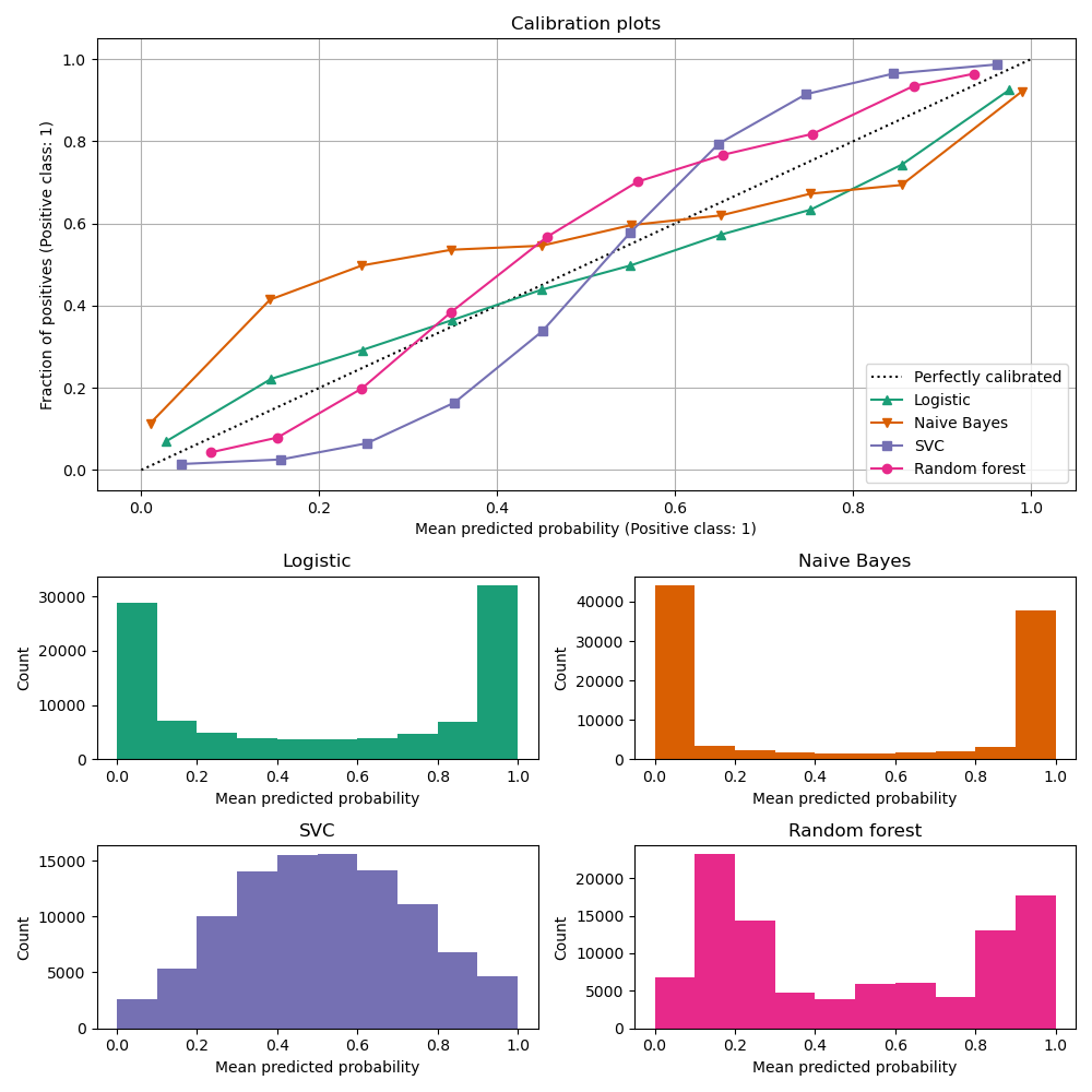{fig-align="center"} :::footer [code](https://scikit-learn.org/stable/modules/calibration.html) ::: ## Calibration metrics Let $N$ be the total of samples, $B$ the number of binds, $n^b$ the samples in bin $b$, and $conf(b)$ the average predicted probability in bin $b$. - Expected Calibration Error: $$ECE = \sum_{b=1}^B \frac{n^b}{N}|acc(b) - conf(b)|$$ - Maximum Calibration Error: $$MCE = \underset{m \in \{1,2,\dots,|B|\}}{\text{max}} |acc(b) - conf(b)|$$ ## Calibration of modern models 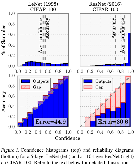{fig-align="center"} :::footer Image taken from Guo, C., Pleiss, G., Sun, Y., & Weinberger, K. Q. (2017, July). *On calibration of modern neural networks. In International Conference on Machine Learning*. PMLR. ::: ## Calibration of modern models 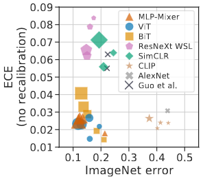{.absolute top="180" left="0" width="330" height="330"} 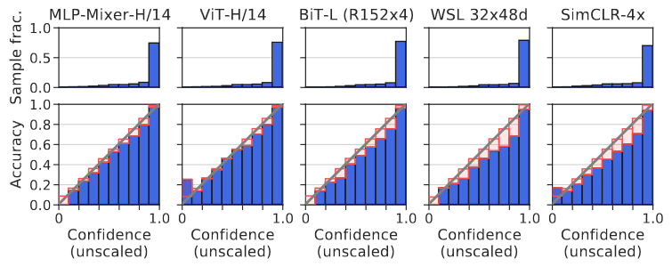{.absolute top="170" left="330" width="800" height="350"} :::footer Image taken from Minderer, Matthias, et al. (2021). *Revisiting the calibration of modern neural networks*. Advances in Neural Information Processing Systems. ::: ## Proper Scoring Rules * Proper scoring rules are calculated at the observation level, where as ECE is binned * Think of them as putting each item in its separate bin, then computing the average of some loss for each predicted probability and its corresponding observed label {fig-align="center"} ::: footer Slides based on [classifier-calibration.github.io](https://classifier-calibration.github.io/) ::: ## Proper Scoring Rules * Brier Score/Quadratic error/Euclidean distance: $$BS = \frac{1}{N} \sum_{i=1}^N (\hat{y}_i - y_i)^2$$ * Log-loss/Cross entropy: - Frequently used to as the training loss of machine learning methods, such as neural networks - Only penalises the probability given to the true class $$LL = -\frac{1}{N} \sum_{i=1}^N [y_i \text{log}(\hat{y}_i) + (1-y_i)\text{log}( 1 - \hat{y}_i)]$$ ::: footer Slides based on [classifier-calibration.github.io](https://classifier-calibration.github.io/) ::: ## Proper Scoring Rules An intuitive way to decompose proper scoring rules is into refinement and calibration losses * **Refinement loss:** is the loss due to producing the same probability for instances from different classes * **Calibration loss:** is the loss due to the difference between the probabilities predicted by the model and the proportion of positives among instances with the same output ::: footer Slides based on [classifier-calibration.github.io](https://classifier-calibration.github.io/) ::: ## Calibration Techniques **Parametric** calibration involves modelling the score distributions within each class - **Platt scaling:** Logistic calibration can be derived by assuming that the scores within both classes are normally distributed with the same variance (Platt, 2000) - **Beta calibration:** employs Beta distributions instead, to deal with scores already on a [0, 1] scale (Kull et al., 2017) - **Dirichlet calibration** for more than two classes (Kull et al., 2019) **Non-parametric** calibration often ignores scores and employs ranks - **Isotonic regression** fits a non-parametric isotonic regressor, which outputs a step-wise non-decreasing function ::: footer Slides based on [classifier-calibration.github.io](https://classifier-calibration.github.io/) ::: ## Platt scaling * Assumes the calibration curve can be corrected by applying a sigmoid to the raw predictions. This means finding $\mathbf{A}$ and $\mathbf{b}$ via MLE: $$p(y_i = 1 | \hat{y}_i) = \frac{1}{1 + exp(\mathbf{A}\hat{y}_i + \mathbf{b})}$$ * Works best if the calibration error is symmetrical (classifier output for each binary class is normally distributed with the same variance) * This can be a problem for highly imbalanced classification problems, where outputs do not have equal variance * In general it is most effective when the un-calibrated model is under-confident and has similar calibration errors for both high and low outputs ## Isotonic regression * Fits a non-parametric isotonic regressor, which outputs a step-wise non-decreasing function * Isotonic regression is more general when compared to Platt scaling, as the only restriction is that the mapping function is monotonically increasing * Is more powerful as it can correct any monotonic distortion of the un-calibrated model * However, it is more prone to overfitting, especially on small datasets ## Calibration in sklearn {fig-align="center"} :::footer [code](https://scikit-learn.org/stable/auto_examples/calibration/plot_calibration_curve.html) ::: ## Calibration in sklearn 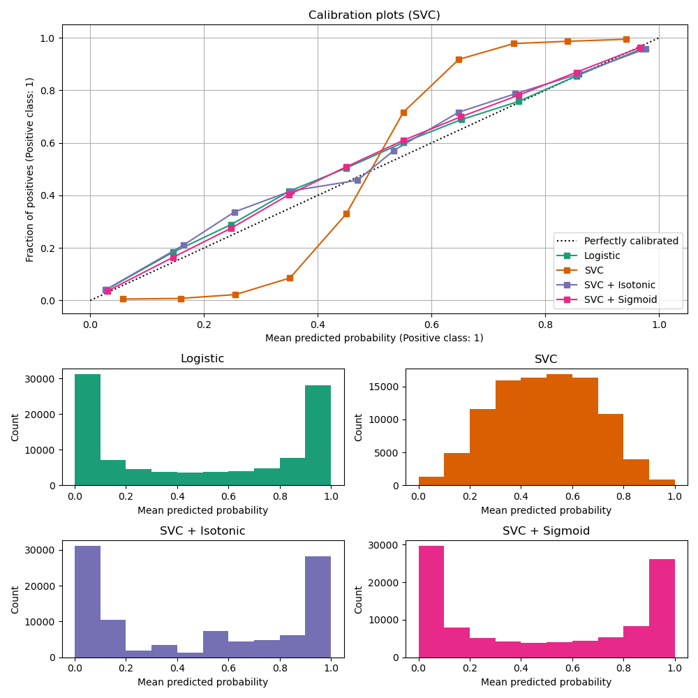{fig-align="center"} :::footer [code](https://scikit-learn.org/stable/auto_examples/calibration/plot_calibration_curve.html) ::: ## Calibration Takeaways * Reliability diagrams are a standard way to visualize calibration * ECE is a summary of what reliability diagrams show * Proper scoring rules (Log loss, Brier score) measure different aspects of probability correctness * However, proper scoring rules cannot tell us where a model is miscalibrated ## Hyperparameters of reliability diagrams \ 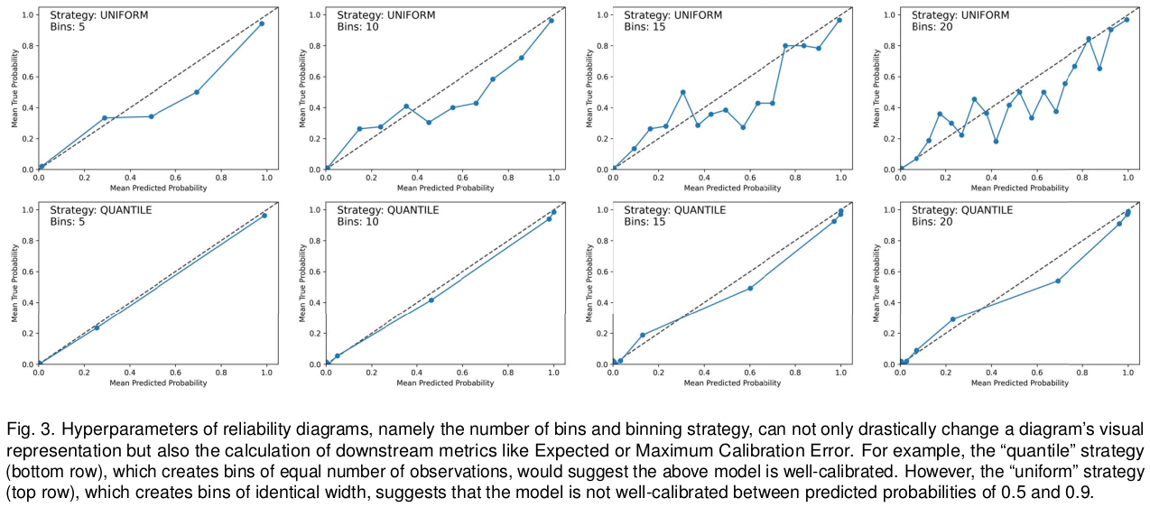{fig-align="center"} :::footer Image taken from Xenopoulos, P., Rulff, J., Nonato, L. G., Barr, B., & Silva, C. (2022). *Calibrate: Interactive analysis of probabilistic model output*. IEEE Transactions on Visualization and Computer Graphics. ::: ## Calibrate (2023) 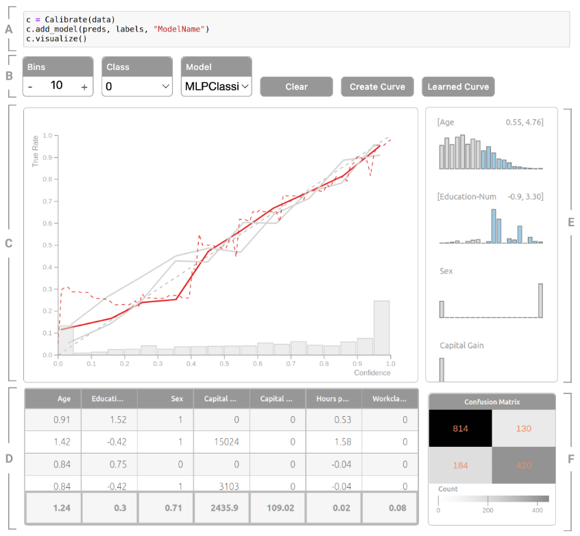{fig-align="center"} :::footer Xenopoulos, P., Rulff, J., Nonato, L. G., Barr, B., & Silva, C. (2022). *Calibrate: Interactive analysis of probabilistic model output*. IEEE Transactions on Visualization and Computer Graphics. ::: ## Calibrate (2023) - Learned Reliability Diagram 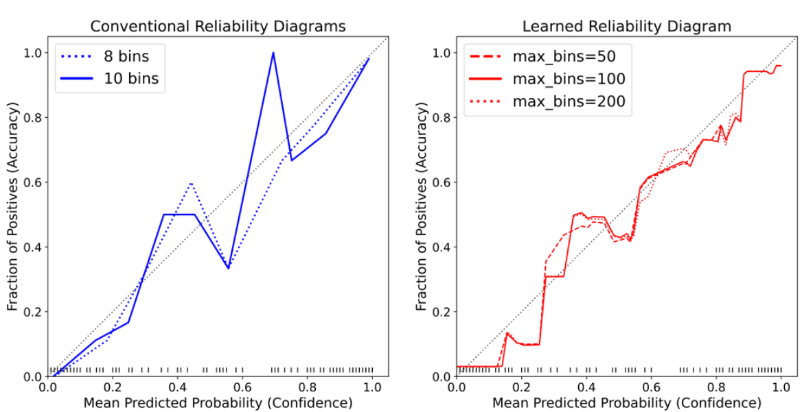{fig-align="center"} :::footer Xenopoulos, P., Rulff, J., Nonato, L. G., Barr, B., & Silva, C. (2022). *Calibrate: Interactive analysis of probabilistic model output*. IEEE Transactions on Visualization and Computer Graphics. ::: ## Calibrate (2023) :::footer Xenopoulos, P., Rulff, J., Nonato, L. G., Barr, B., & Silva, C. (2022). *Calibrate: Interactive analysis of probabilistic model output*. IEEE Transactions on Visualization and Computer Graphics. ::: ## Smooth ECE (2023) \ 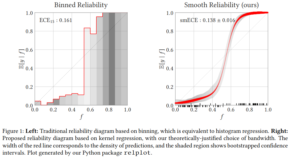{fig-align="center"} :::footer Błasiok, J., & Nakkiran, P. (2023). *Smooth ECE: Principled Reliability Diagrams via Kernel Smoothing*. arXiv preprint arXiv:2309.12236. ::: ## Smooth ECE (2023) \ 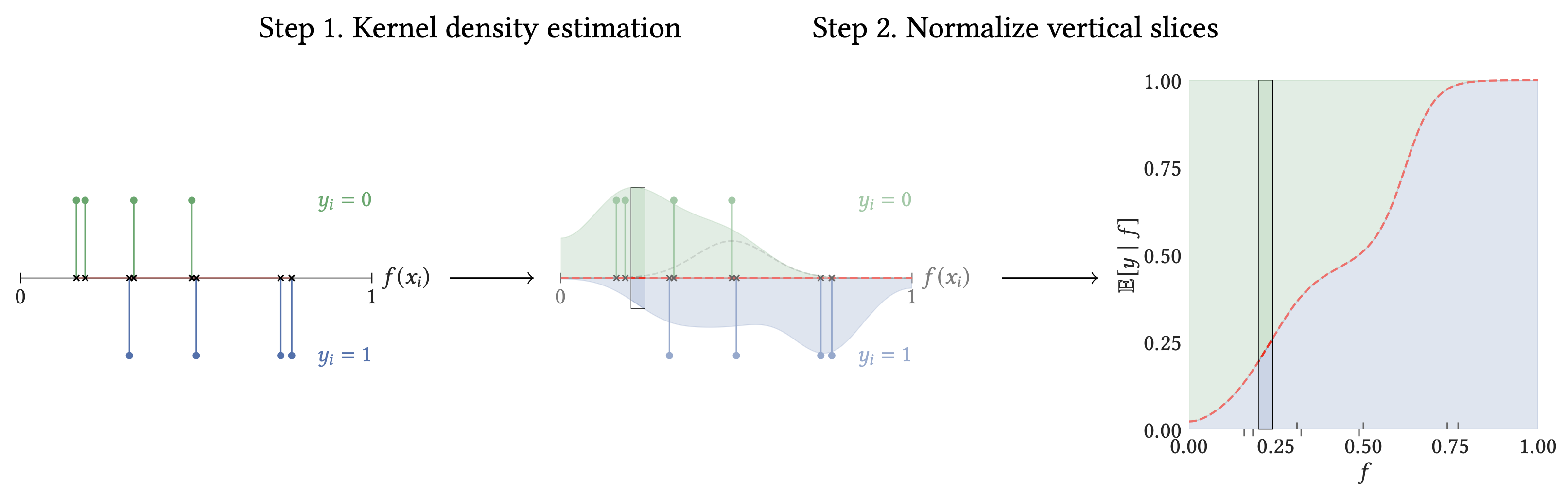{fig-align="center"} :::footer Błasiok, J., & Nakkiran, P. (2023). *Smooth ECE: Principled Reliability Diagrams via Kernel Smoothing*. arXiv preprint arXiv:2309.12236. ::: ## Visualizing Calibration for Multi-Class Problems 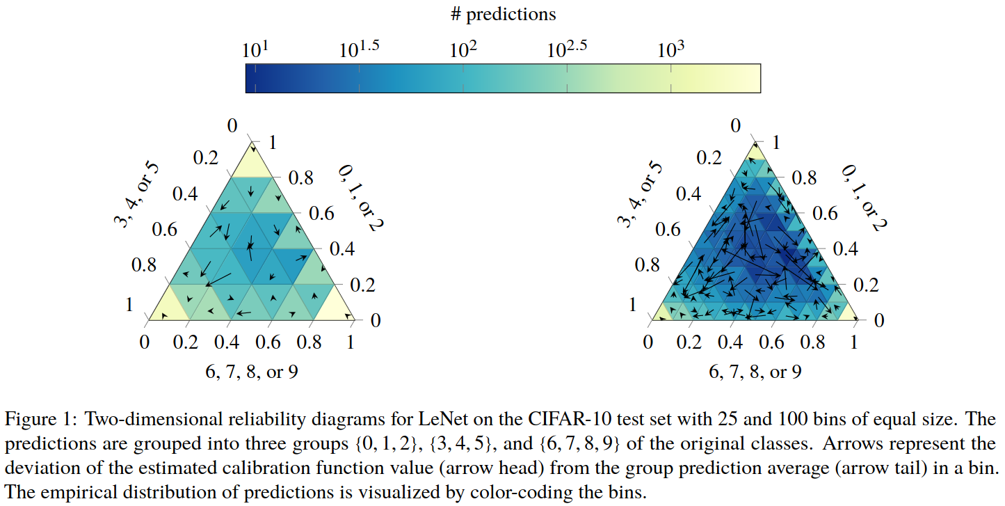{fig-align="center"} :::footer Image taken from Vaicenavicius, Juozas, et al. *Evaluating model calibration in classification*. The 22nd International Conference on Artificial Intelligence and Statistics. PMLR, 2019. ::: ## Suggested Calibration Literature * Niculescu-Mizil, A., & Caruana, R. (2005, August). [Predicting good probabilities with supervised learning](https://dl.acm.org/doi/pdf/10.1145/1102351.1102430?casa_token=o_8UMED_0fIAAAAA:MIq2GzQTPT0f-aWNDSijbcnzJN1riBdGqjq9FGn-wOZ188AOtXbTqRPkc9PuQGKSFIo5b4fM8-ItjQ). In Proceedings of the 22nd international conference on Machine learning (pp. 625-632). * Nixon, J., Dusenberry, M. W., Zhang, L., Jerfel, G., & Tran, D. (2019, June). [Measuring Calibration in Deep Learning](http://openaccess.thecvf.com/content_CVPRW_2019/papers/Uncertainty%20and%20Robustness%20in%20Deep%20Visual%20Learning/Nixon_Measuring_Calibration_in_Deep_Learning_CVPRW_2019_paper.pdf). In CVPR Workshops (Vol. 2, No. 7). * Guo, C., Pleiss, G., Sun, Y., & Weinberger, K. Q. (2017, July). [On calibration of modern neural networks](http://proceedings.mlr.press/v70/guo17a/guo17a.pdf). In International Conference on Machine Learning (pp. 1321-1330). PMLR. * Vaicenavicius, J., Widmann, D., Andersson, C., Lindsten, F., Roll, J., & Schön, T. (2019, April). [Evaluating model calibration in classification](http://proceedings.mlr.press/v89/vaicenavicius19a/vaicenavicius19a.pdf). In The 22nd International Conference on Artificial Intelligence and Statistics (pp. 3459-3467). PMLR. ## Suggested Calibration Literature * Kull, M., & Flach, P. (2015, September). [Novel decompositions of proper scoring rules for classification: Score adjustment as precursor to calibration](https://link.springer.com/content/pdf/10.1007/978-3-319-23528-8_5.pdf). In Joint European Conference on Machine Learning and Knowledge Discovery in Databases (pp. 68-85). Springer, Cham. * [ECML/PKDD 2020 Tutorial: Evaluation metrics and proper scoring rules](https://classifier-calibration.github.io/assets/slides/clacal_tutorial_ecmlpkdd_2020_evaluation.pdf) * [Google Colab notebook for calibration curves](https://colab.research.google.com/drive/1mqDVJICMBg2eoIr2VPaDjQFUzlDT3grc?usp=sharing)