Visualization for Machine Learning
Spring 2024
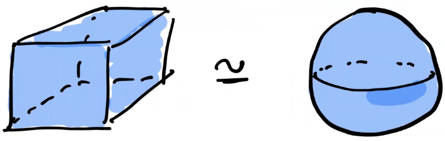
What is topology?
Topology studies the shape of mathematical objects
Unlike Geometry, it is not concerned with sizes, angles, nor coordinates
It is concerned with the connectivity (or lack of) between different “parts” of the object
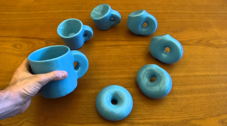
Two objects are topologically equivalent if we can transform one into another with continuous transformations (without tearing the object)
What is topology?
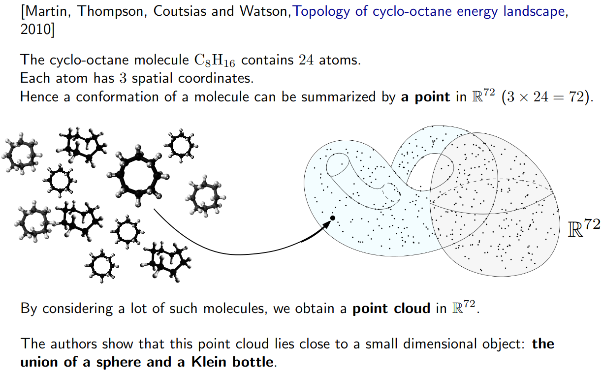
Why topology? - An example in chemistry
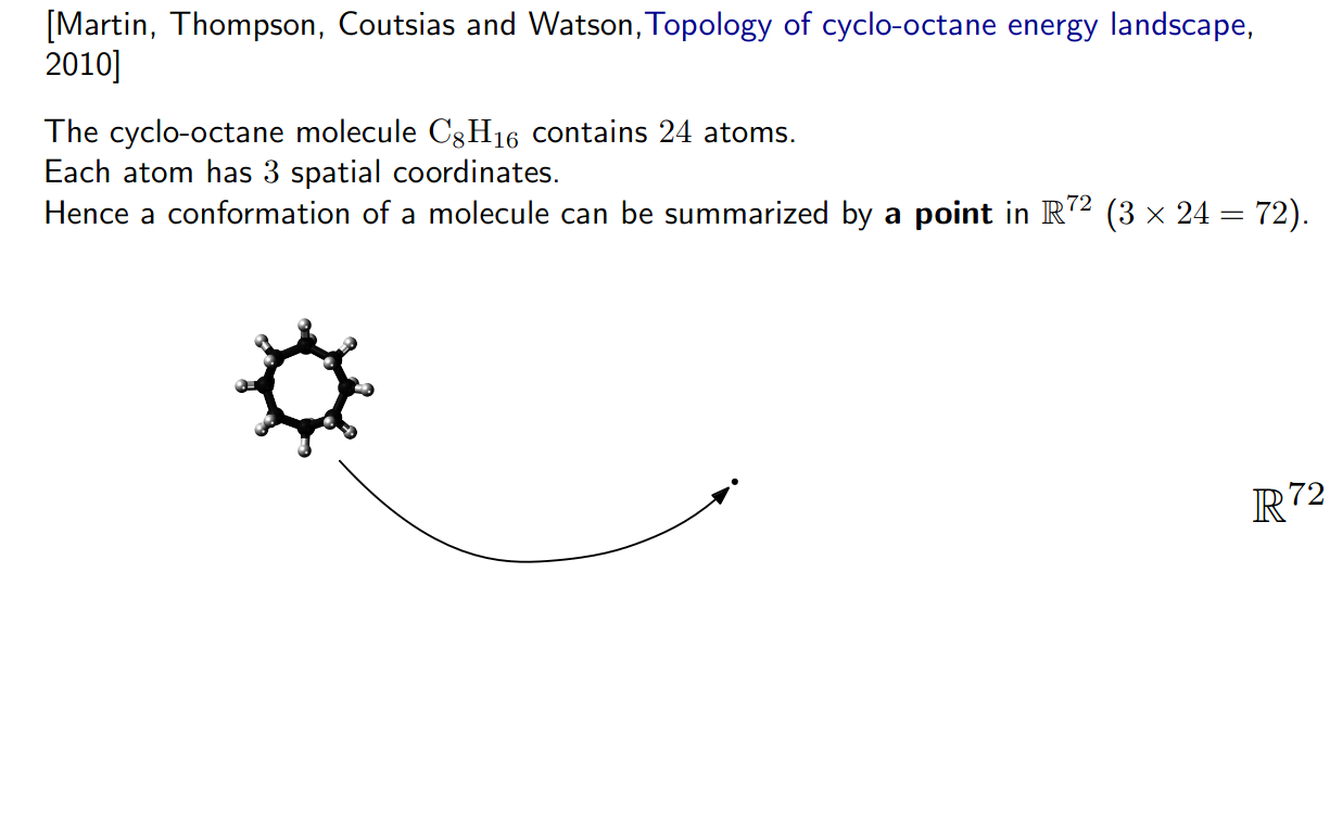
Why topology? - An example in chemistry
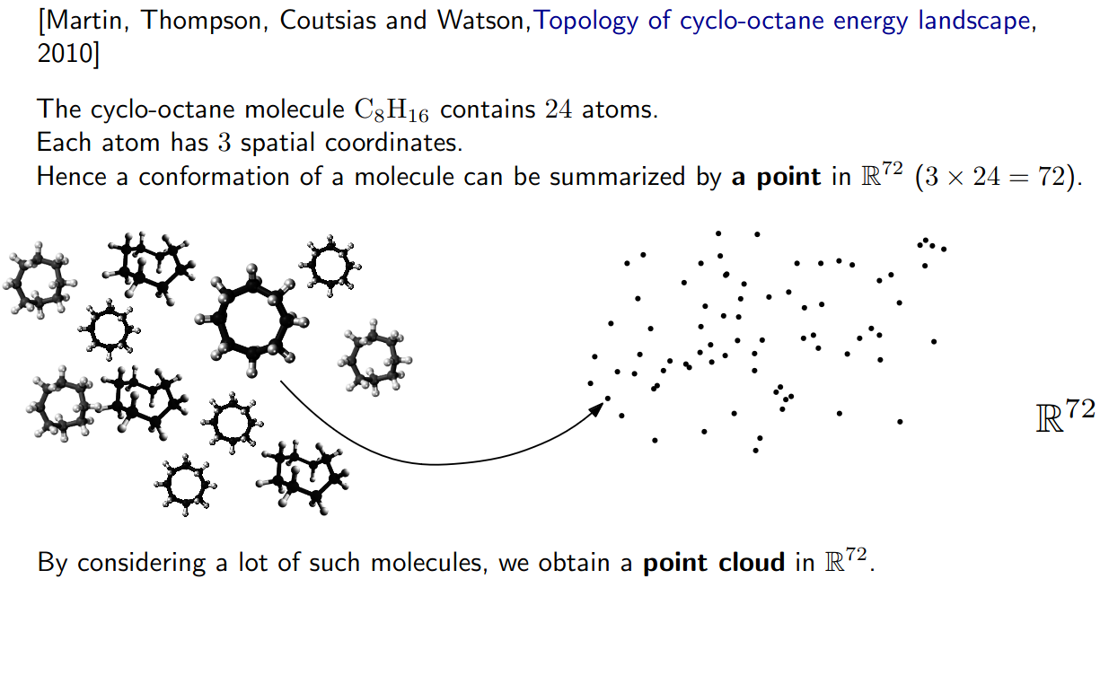
Why topology? - An example in chemistry
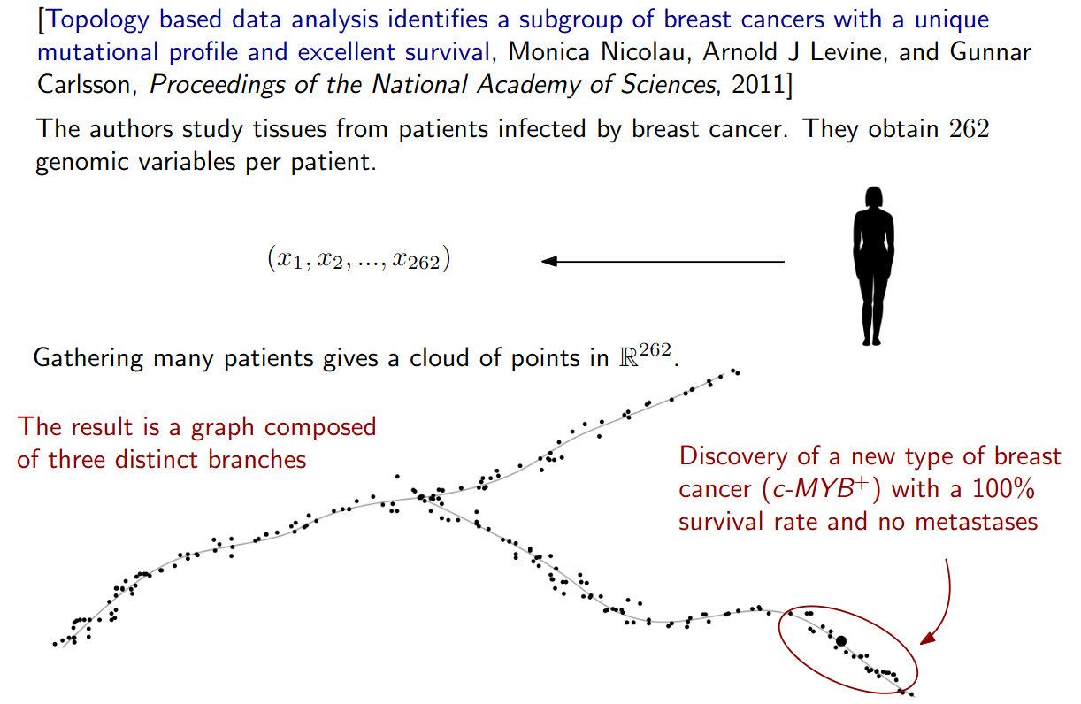
Why topology? - An example in biology
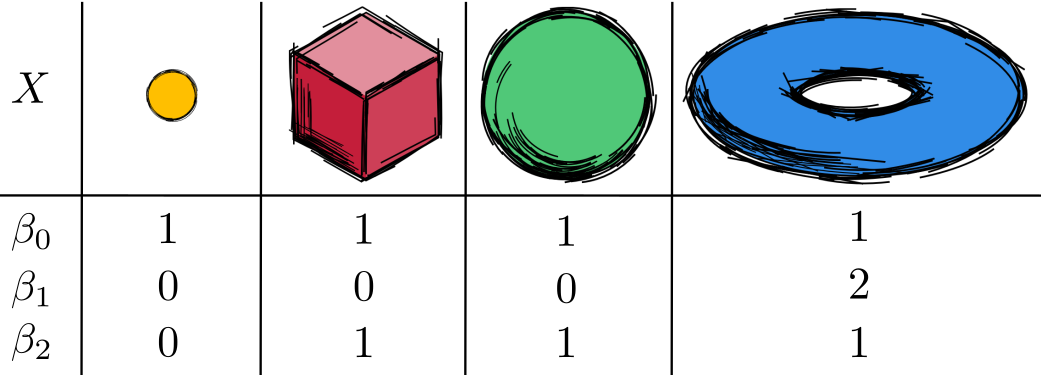
Betti numbers
The \(d^{th}\) Betti number counts the number of \(d\)-dimensional holes. It can be used to distinguish between spaces.
\(\beta_0(X)\) Connected components in X
\(\beta_1(X)\) Tunnels or holes in X
\(\beta_2(X)\) Voids in X
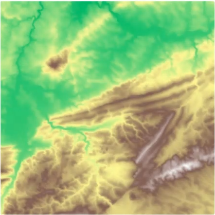
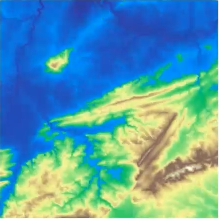
First Example - Map
What is a peak?
First Example - Map
What is a peak?
First idea: Using local maximum
First Example - Map
What is a peak?
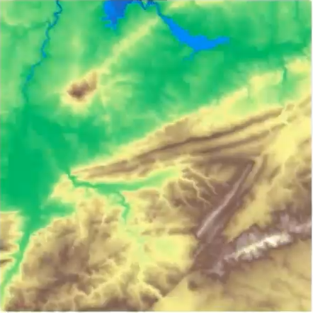
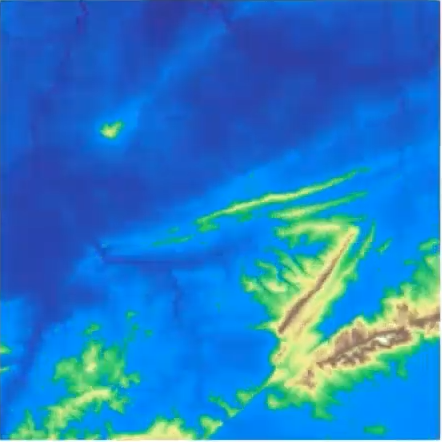
Second idea: flooding
First Example - Map
What is a peak?
Second idea: flooding
First Example - Map
What is a peak?
Second idea: flooding
First Example - Map
What is a peak?
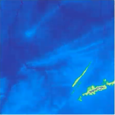
Second idea: flooding
First Example - Map
What is a peak?
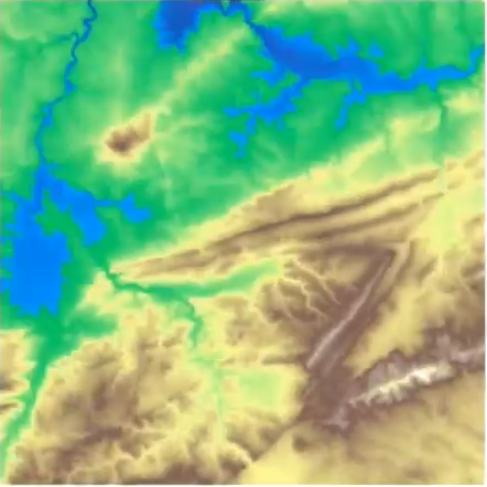
Second idea: flooding
First Example - Map
What is a peak?
Second idea: flooding
First Example - Map
What is a peak?
Second idea: flooding

First Example - Map
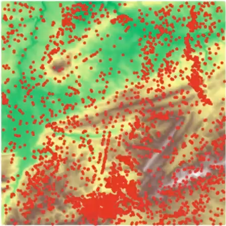
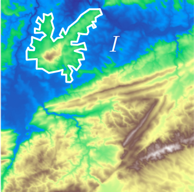
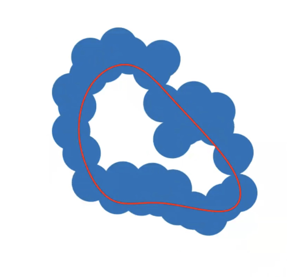
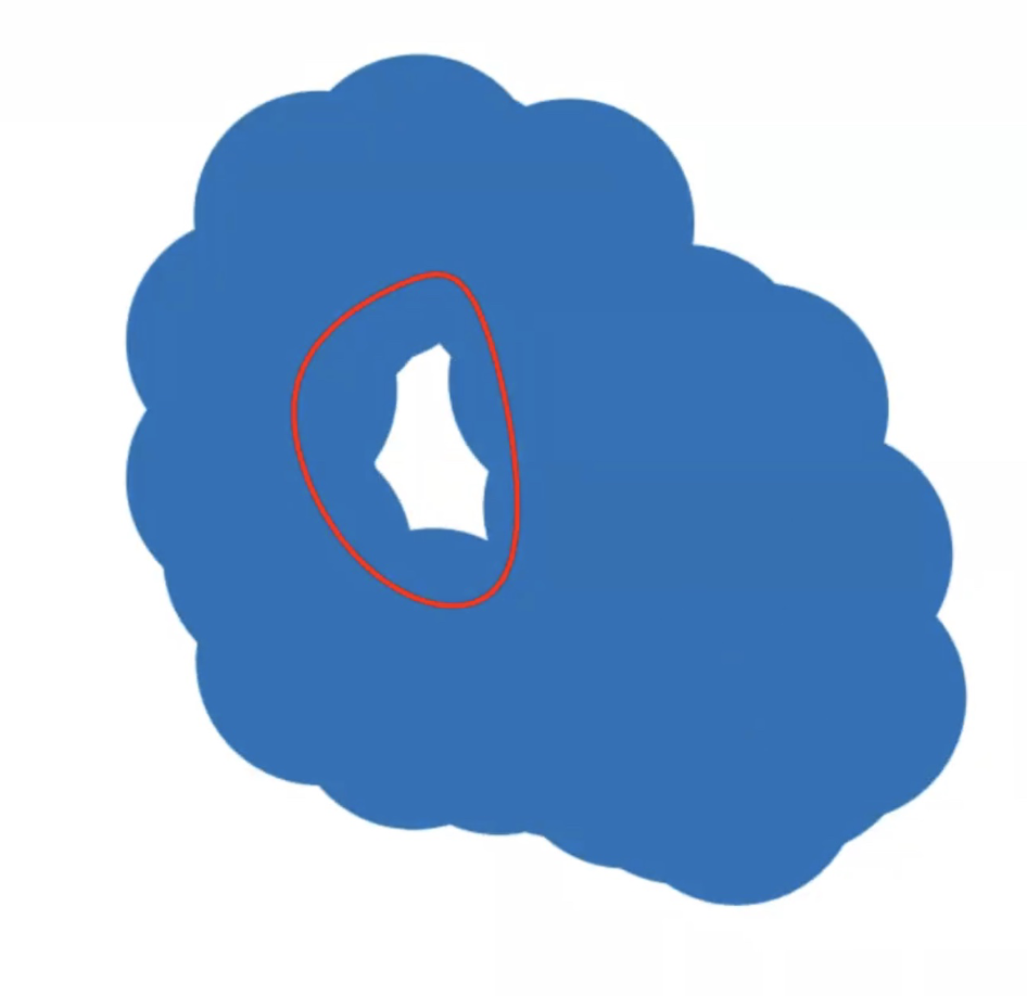
The island \(I\) appears at sea level \(b\) (its birth time)…
First Example - Map
The island \(I\) appears at sea level \(b\) (its birth time)…
and disapears at seas level \(d\) (its death time) at local maximum \(x\).
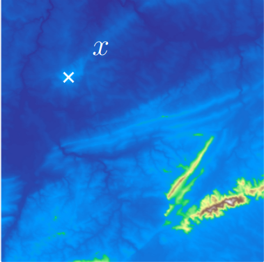
The point \(x\) is a peak if the persistence\(:= d-b\) of the island \(I\) is larger than \(91\)m (=\(300\)ft).
First Example - Map
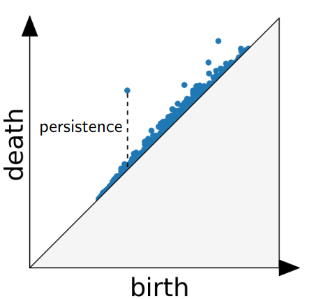
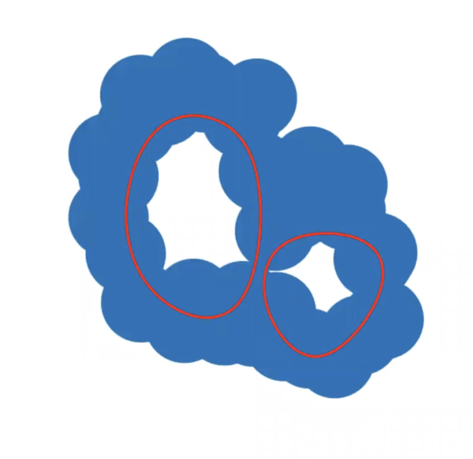
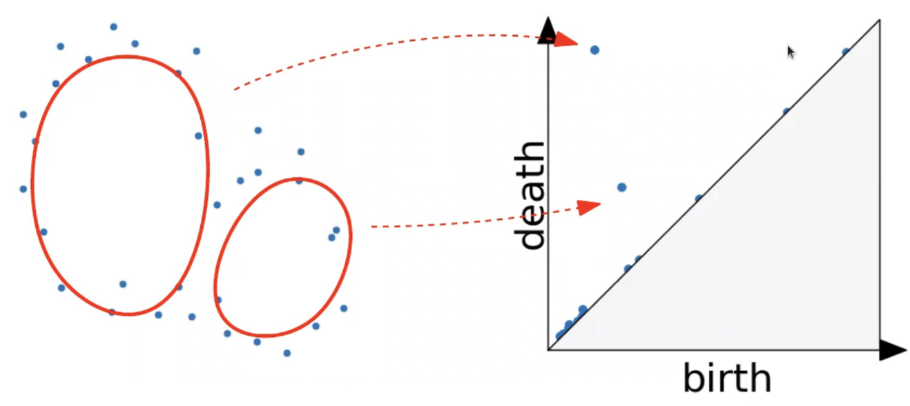
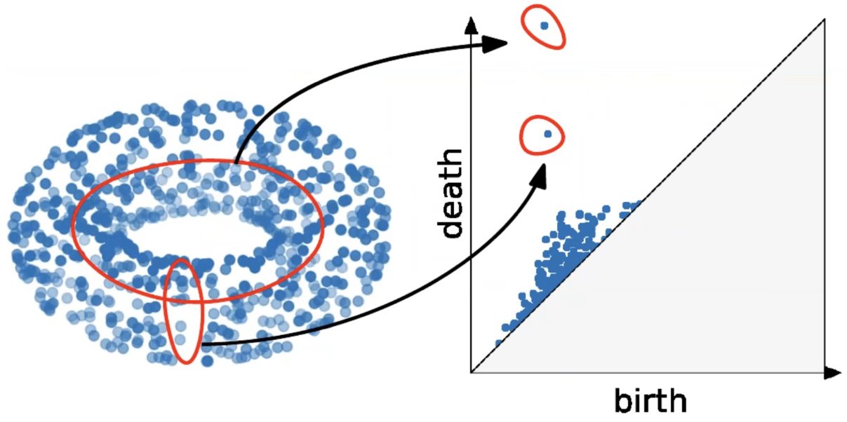
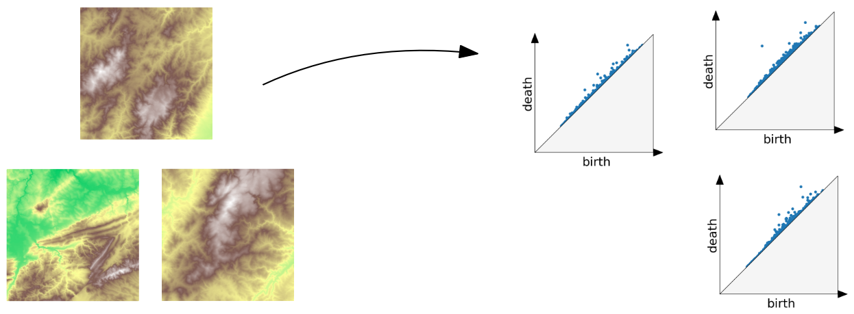
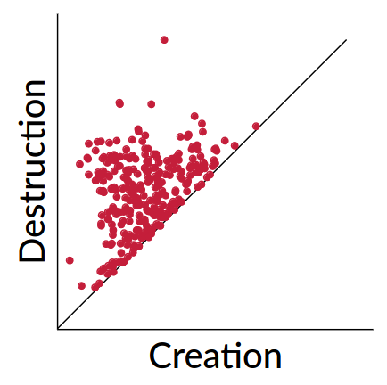
The persistence diagram (PD) of the elevation function is the collection of the points \((b,d)\), where \((b,d)\) corresponds to the birth/death of an island.
First Example - Map
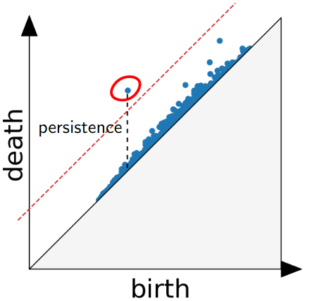
The persistence diagram (PD) of the elevation function is the collection of the points \((b,d)\), where \((b,d)\) corresponds to the birth/death of an island.
Second Example
Second Example
Second Example
Second Example
Second Example
Second Example

Second Example

Second Example

Second Example
Second Example
Second Example
Second Example

Second Example
Persistence diagram
Distance between persistence diagrams
If we have more than one persistence diagram, how do we measure the distance between them?
Distance between persistence diagrams
We place both in the same diagram
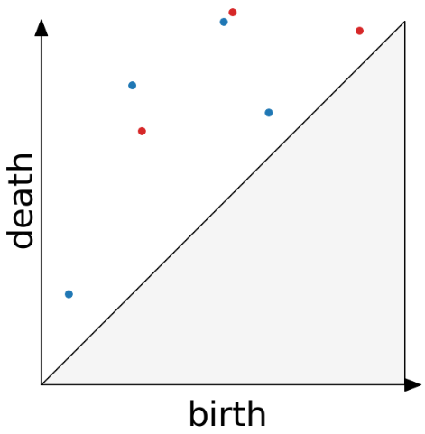
Distance between persistence diagrams
We place both in the same diagram
Get the optimal pair matching between the points (including the diagonal)
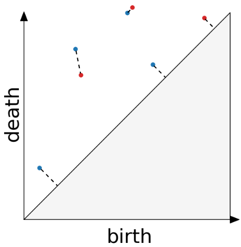
Distance between persistence diagrams
We place both in the same diagram
Get the optimal pair matching between the points (including the diagonal)
The bottleneck distance between them will be the largest pair distance
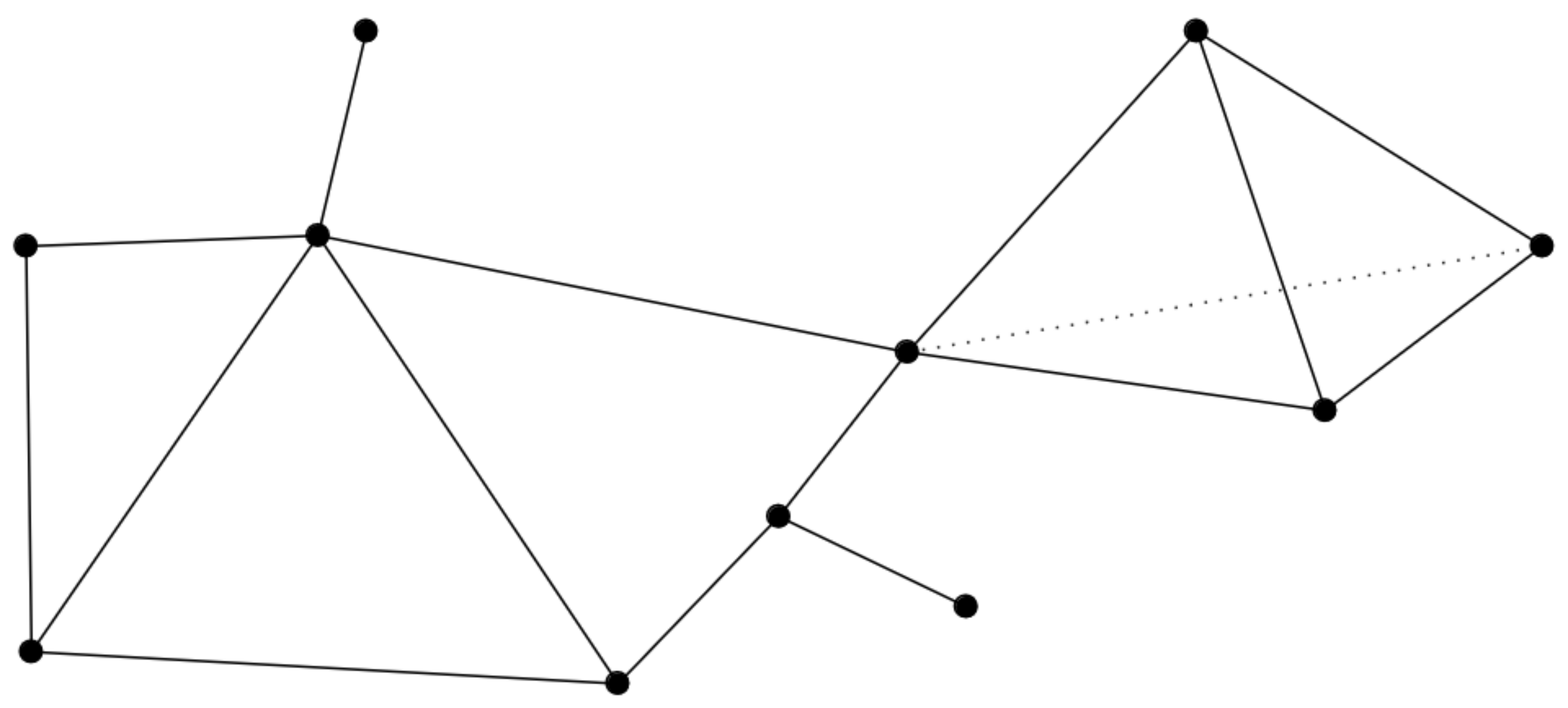
Simplicial complexes
Example
Simplicial complexes can be decomposed into their skeletons, which only contain simplices of a certain dimension.
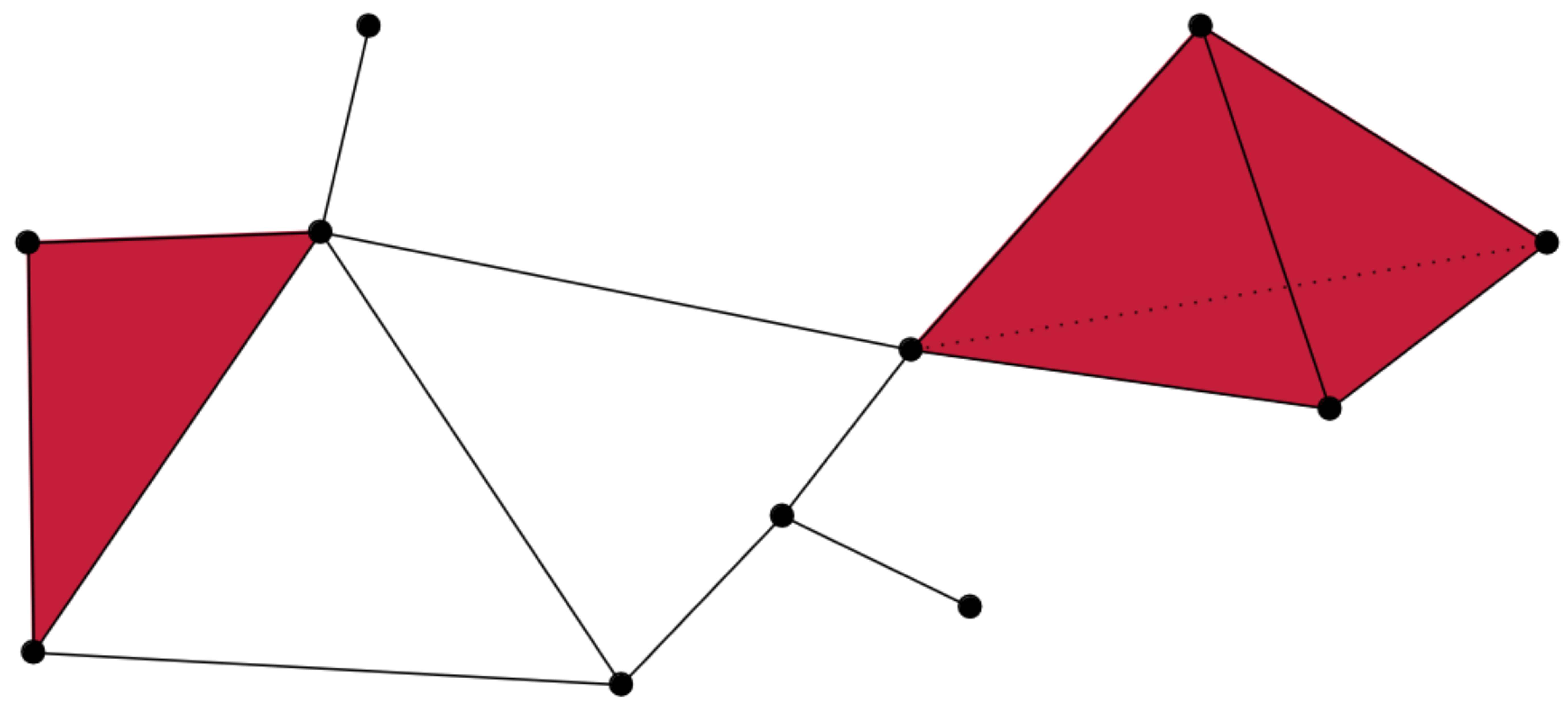
Simplicial complexes
Example
Simplicial complexes can be decomposed into their skeletons, which only contain simplices of a certain dimension.
Simplicial complexes
Example
Simplicial complexes can be decomposed into their skeletons, which only contain simplices of a certain dimension.
Simplicial complexes
Example
Simplicial complexes can be decomposed into their skeletons, which only contain simplices of a certain dimension.
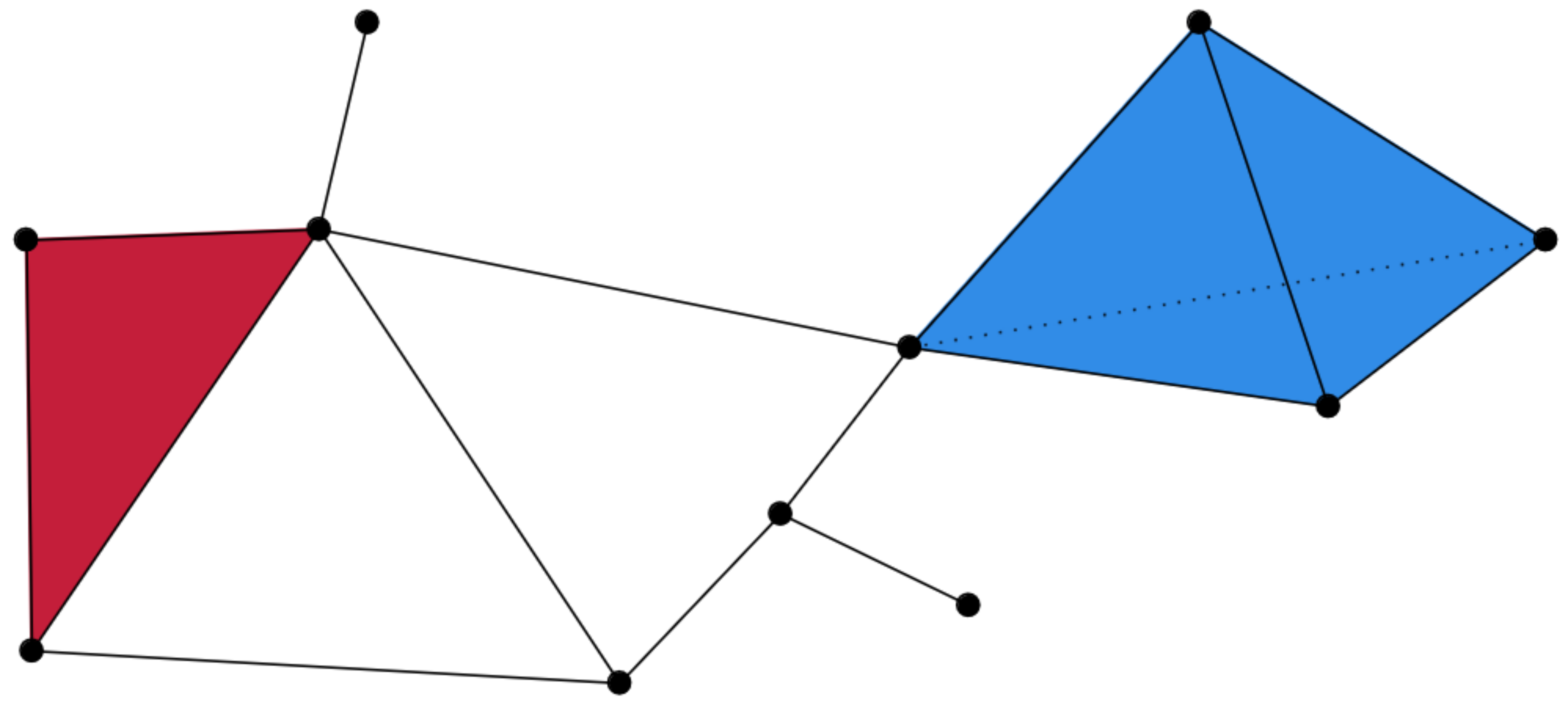
Simplicial complexes
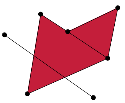
Non-example
This is not a simplicial complex because some higher-dimensional simplices do not intersect in a lower dimensional one!
Simplicial complexes
Example
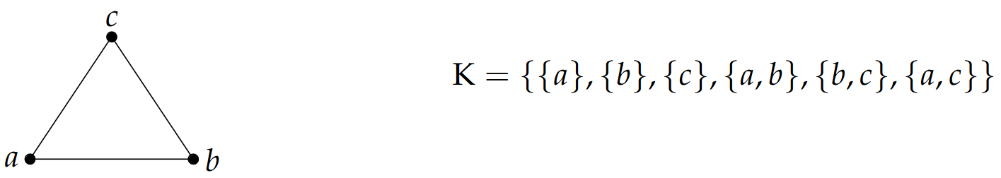
Notice that \(K\) does not contain the 2-simplex \(\{a,b,c\}\)
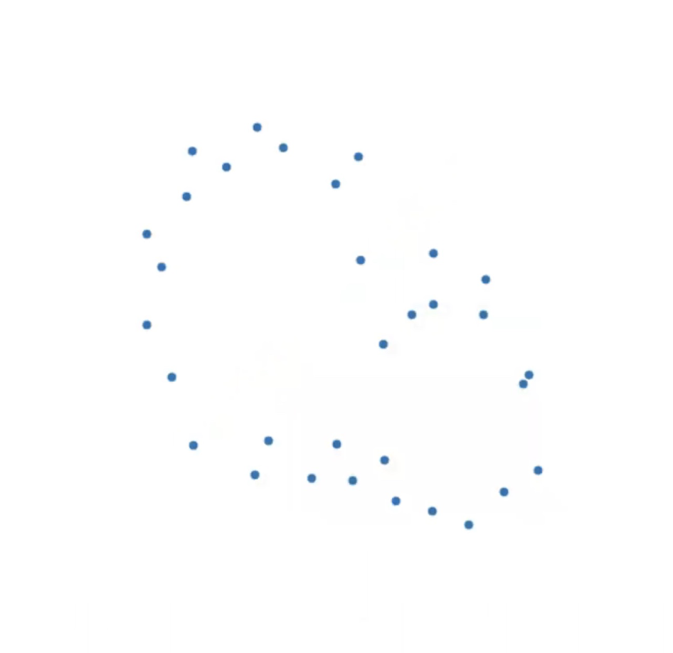
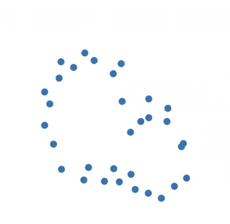
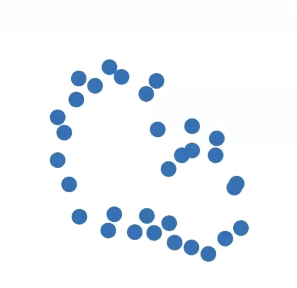
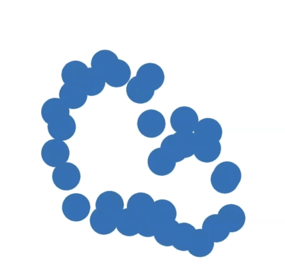
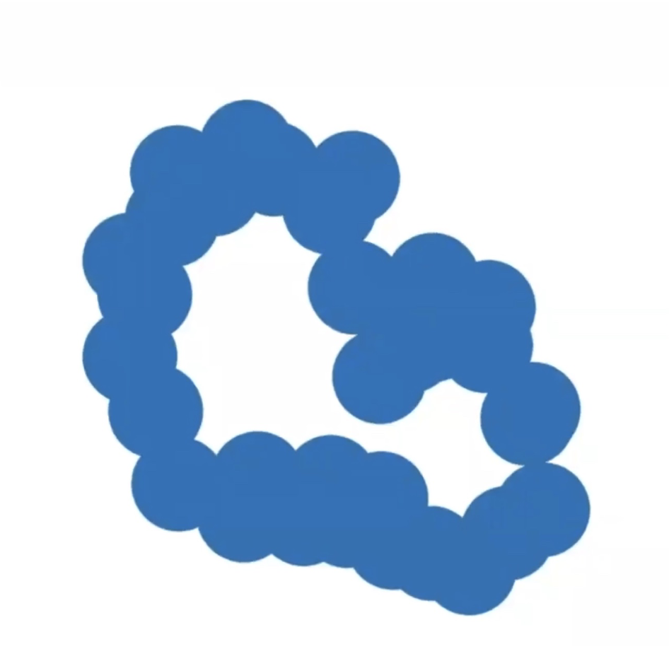
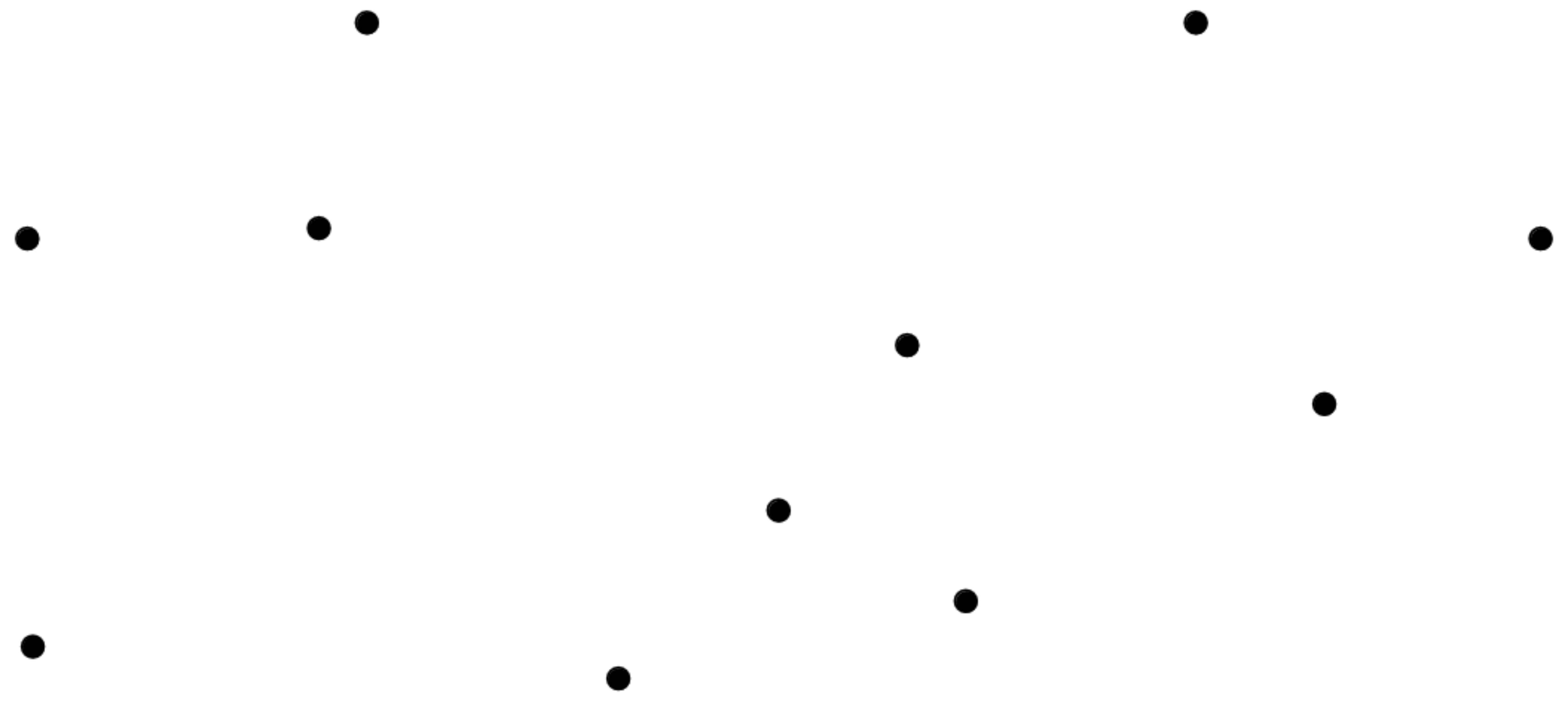
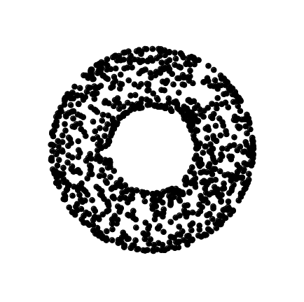
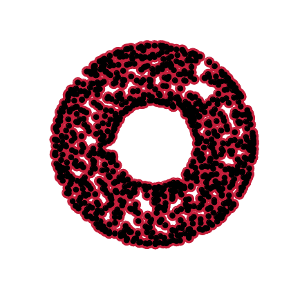
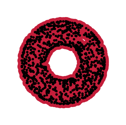
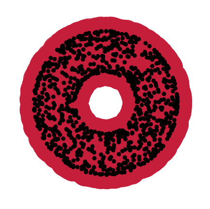
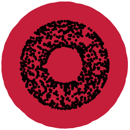
From points clouds to simplicial complexes
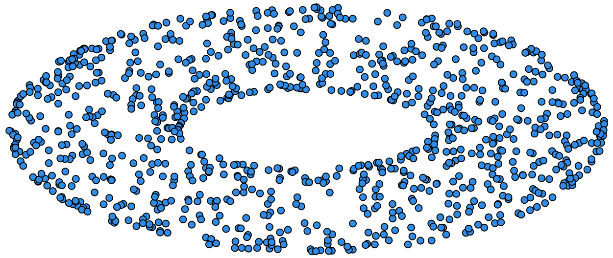
From points clouds to simplicial complexes
Vietoris-Rips construction
Example
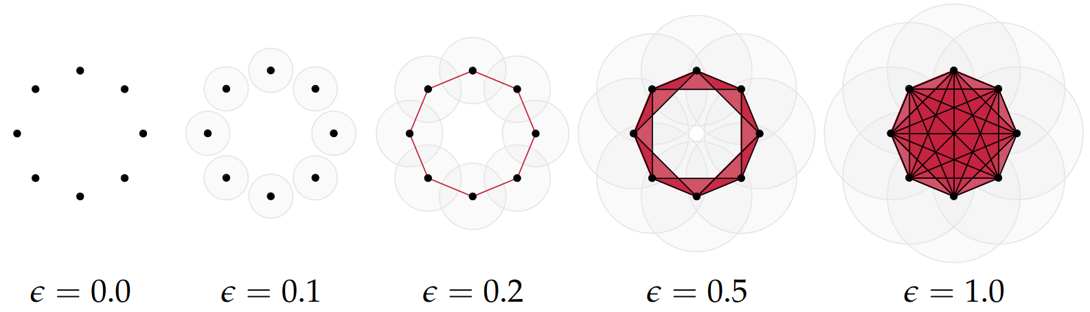
Draw Euclidean balls (circles) of diameter \(\epsilon\) and create a \(k\)-simplex \(\sigma\) for each subset of \(k+1\) points that intersect pairwise.
Some details about this construction
This construction dates back to a 1927 article by Leopold Vietoris\(^1\)
A 2010 paper by Afra Zomorodian\(^2\) describes several construction algorithms
The basic idea is to build higher-dimensional simplices inductively from lower-dimensional ones
In the worst case, the Vietoris-Rips complex will contain all \(2^n\) subsets of its underluing point clous \(\mathcal{X}\)!
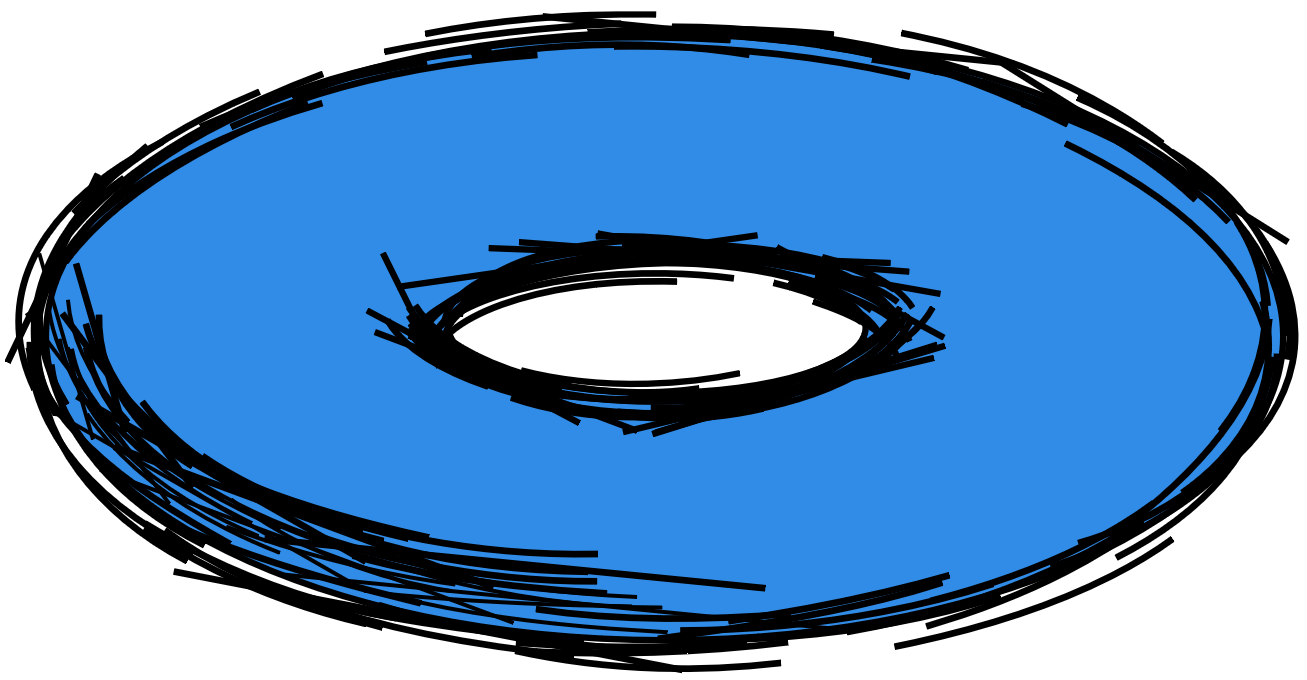
The betti numbers of a Vietoris-Rips complex
Example
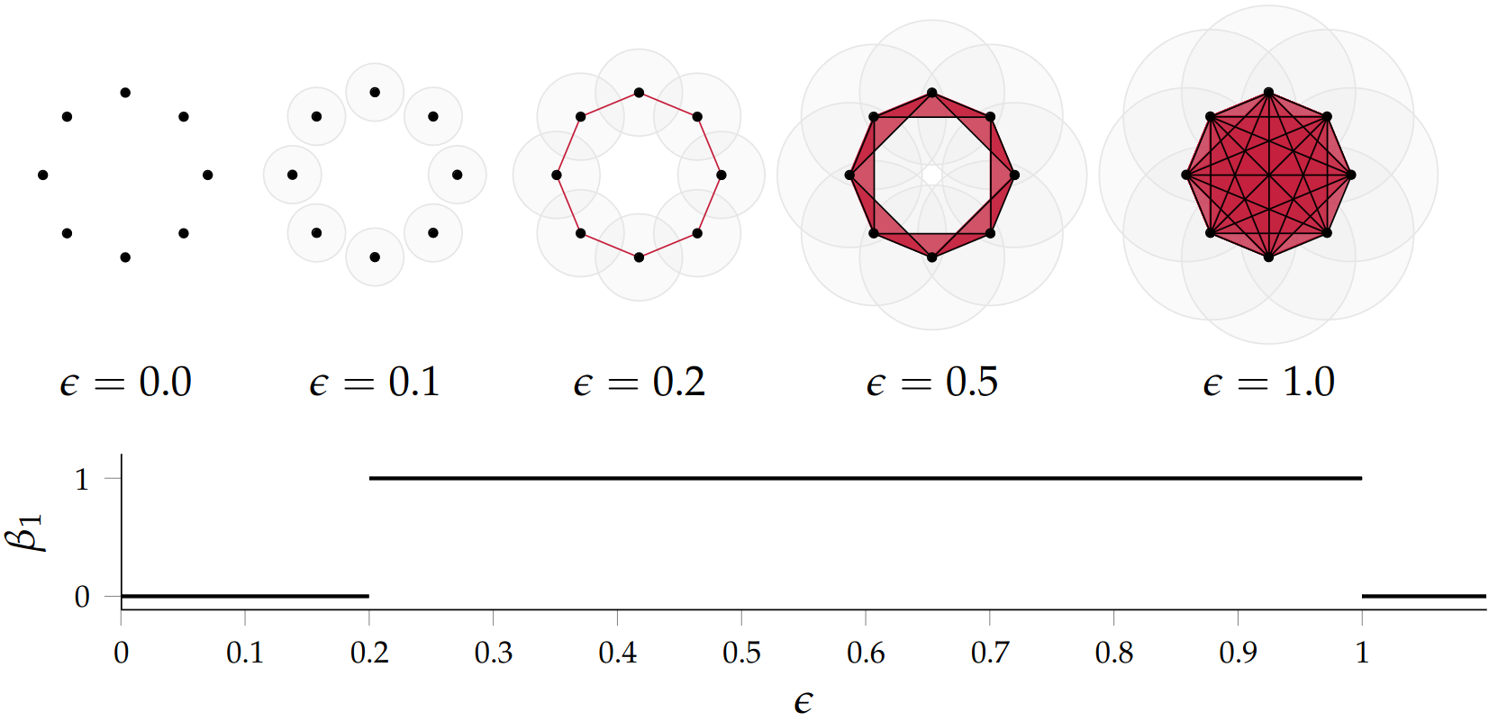
Picking \(\epsilon\) - Topological Persistence
Intuition: Go through all scales and track the topological features
Picking \(\epsilon\) - Topological Persistence
Intuition: Go through all scales and track the topological features
Picking \(\epsilon\) - Topological Persistence
Intuition: Go through all scales and track the topological features
Picking \(\epsilon\) - Topological Persistence
Intuition: Go through all scales and track the topological features
Picking \(\epsilon\) - Topological Persistence
Intuition: Go through all scales and track the topological features
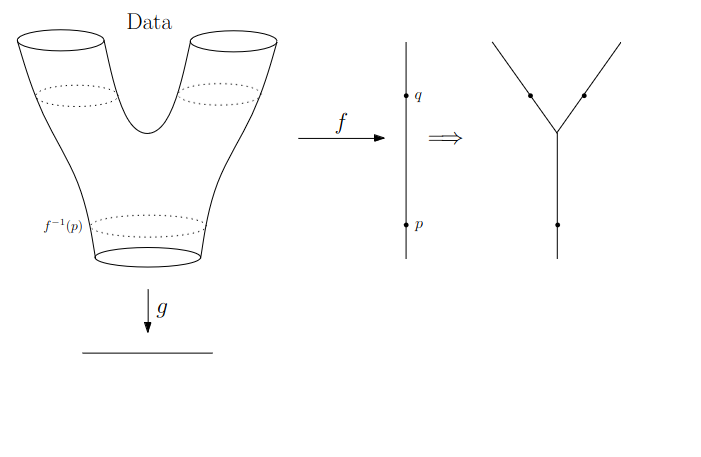
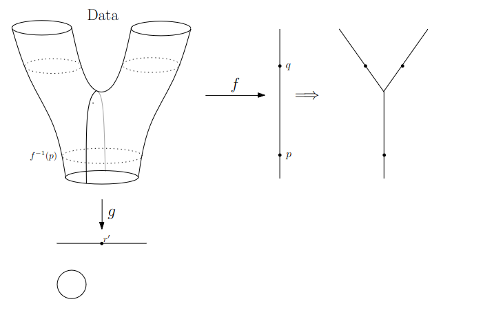
Math World
Math World
Math World
Math World
Math World
Math World
Math World
Math World
Math World
Math World
Math World
Math World
Math World
Math World
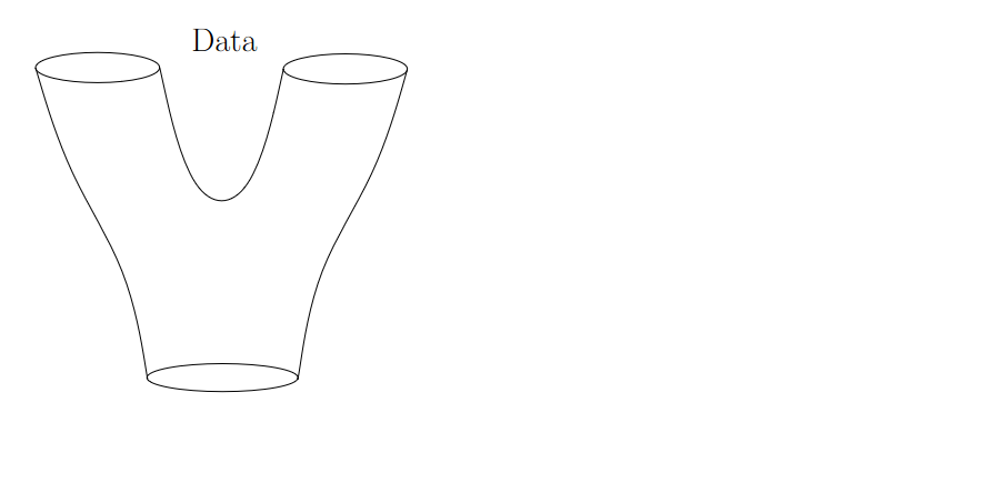
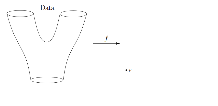
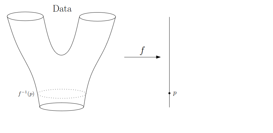
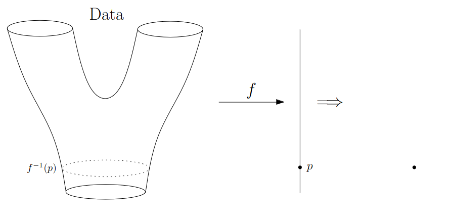
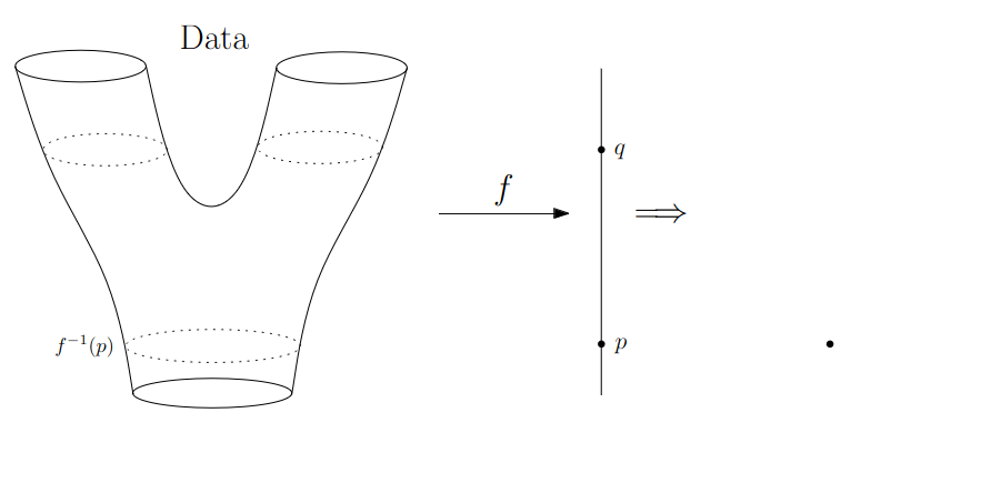
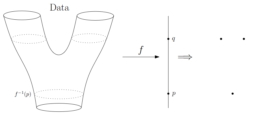
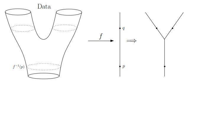
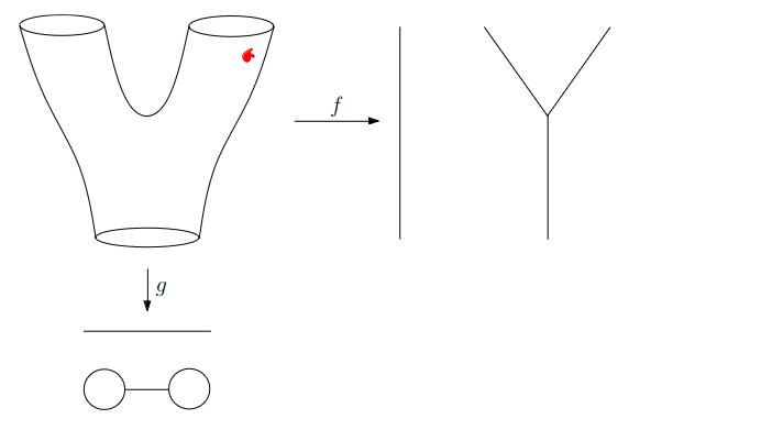
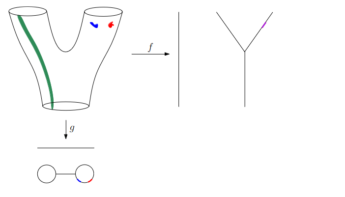
Why is this useful?
We get “easy” understanding of the localizations of quantities of interest.
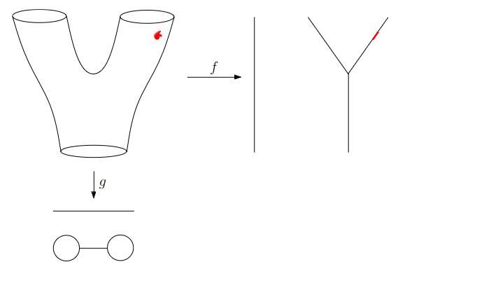
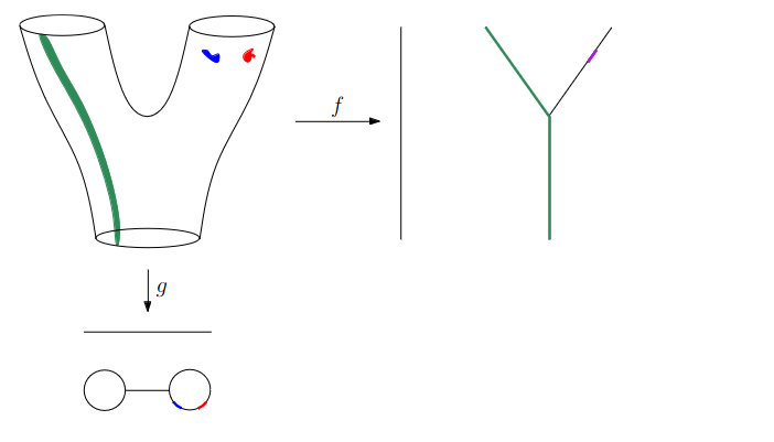
Why is this useful?
We get “easy” understanding of the localizations of quantities of interest.
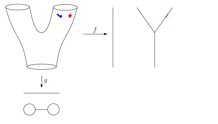
Why is this useful?
We get “easy” understanding of the localizations of quantities of interest.
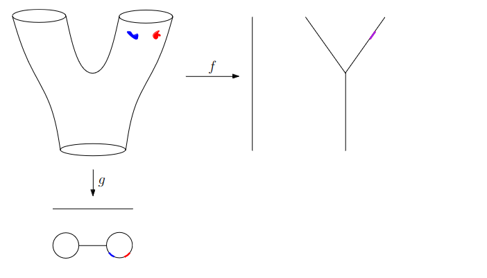
Why is this useful?
We get “easy” understanding of the localizations of quantities of interest.
Why is this useful?
We get “easy” understanding of the localizations of quantities of interest.
Why is this useful?
We get “easy” understanding of the localizations of quantities of interest.
Why is this useful?
We get “easy” understanding of the localizations of quantities of interest.
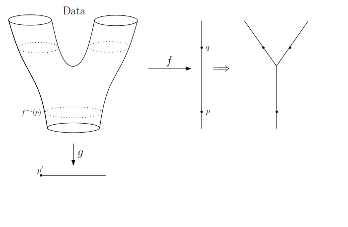
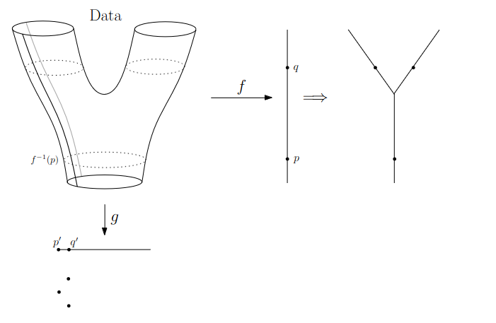
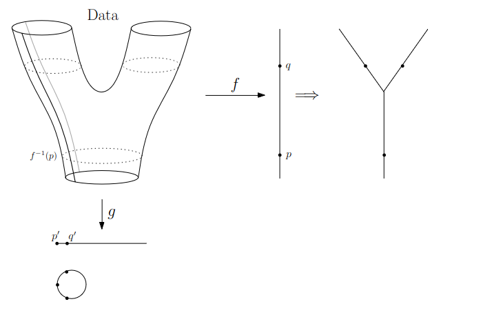
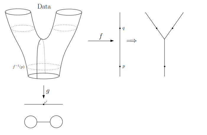
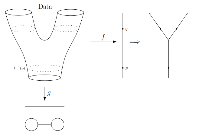
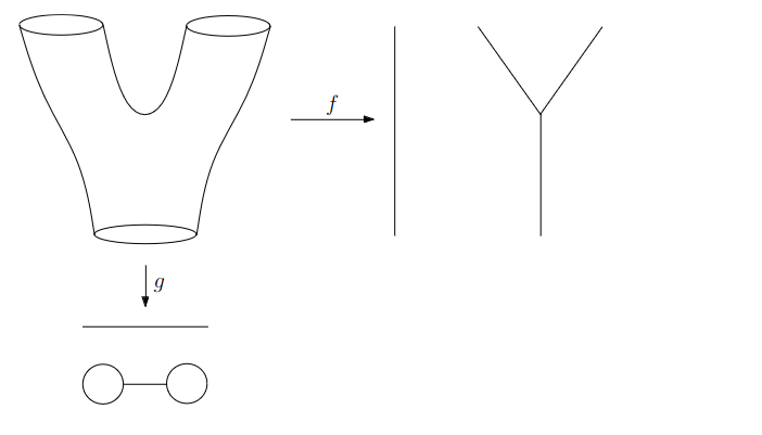
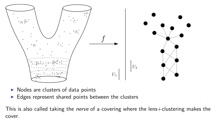
Data World - Mapper
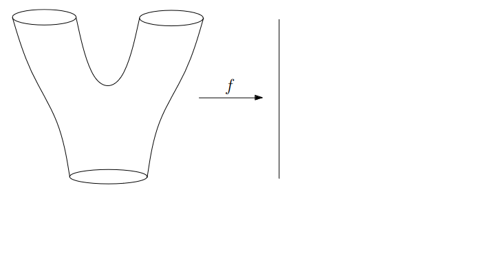
Data World - Mapper
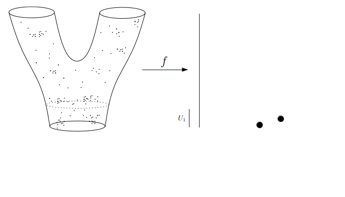
Data World - Mapper
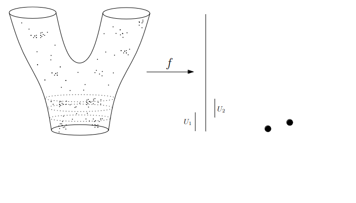
Data World - Mapper
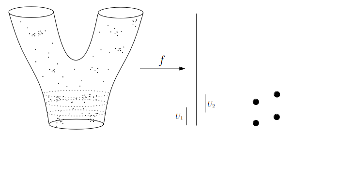
Data World - Mapper

Data World - Mapper
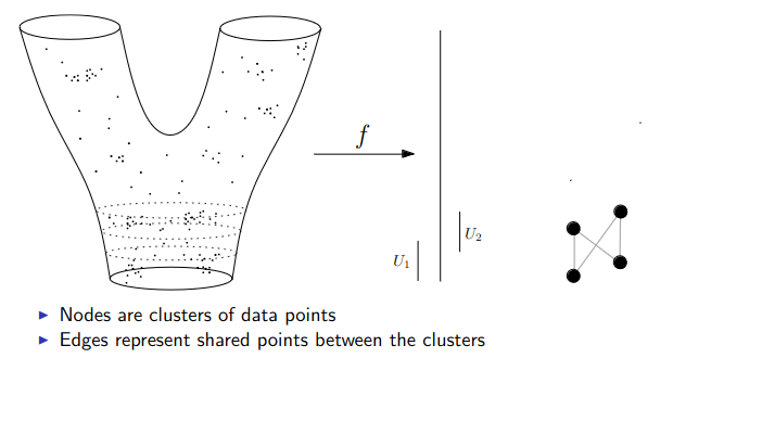
Data World - Mapper
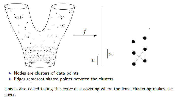
Data World - Mapper
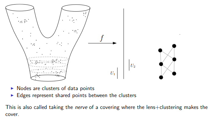
Data World - Mapper

Data World - Mapper
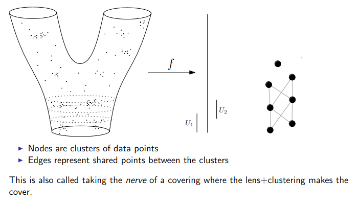
Data World - Mapper
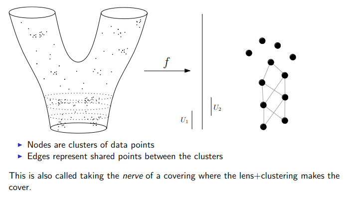
Data World - Mapper
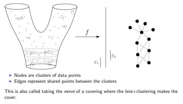
Data World - Mapper
References
TDA in Python:
- For overall TDA data structures and algorithms: GUDHI (both C++ and Python) or scikit-tda
- For a faster implementation of the Vietoris-Rips: Ripser.py
- For a faster implementation of the Mapper: KeplerMapper
For an open-source library and software collection for topological data analysis and visualization: Topology ToolKit
For more examples of TDA aplications:
- DONUT - Database of Original & Non-Theoretical Uses of Topology
- Applied Algebraic Topology Research Network seminar series