Visualization for Machine Learning
Spring 2024
Today’s Class
- Model Interpretation and Explanation
- White-box Approaches and Visualizations
- Related Research in VIS & AI
Today’s Class
- Model Interpretation and Explanation
- White-box Approaches and Visualizations
- Related Research in VIS & AI
Why Model Interpretation & Explanation?
- Model Validation and Improvement
- Decision Making and Knowledge Discovery
- Gain Confidence and Obtain Trust
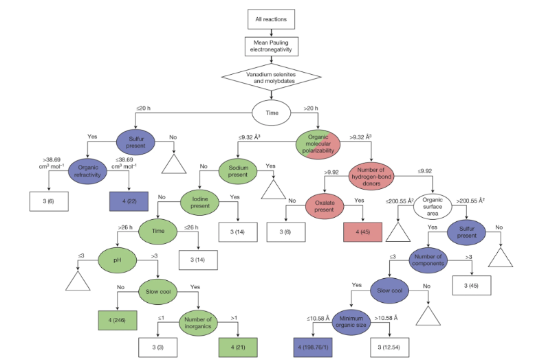
Machine-learning-assisted materials discovery using failed experiments
- Researchers firstly built a database of chemistry experiments (new material).
- Then they train an SVM to predict whether a new chemistry experiment will be successful.
- Then they train a surrogate DT to explain the model to learn more about the experiment.
Why Model Interpretation & Explanation?
- Fairness
- Privacy
- Reliability or Robustness
- Causality
- Trust
How Do We Interpret Model Behavior?
Methods for machine learning model interpretation can be classified according to various criteria.
White-box / Intrinsic interpretability: Machine learning models that are considered interpretable due to their simple structure, such as short decision trees or sparse linear models. Interpretability is gained by explaining the internal structure of the model.
Black-box / Post-hoc interpretability: Machine learning models that are hard to gain a comprehensive understanding of their inner working (e.g., deep neural networks) are considered black boxes. Interpretability is gained by explaining the model behavior after training.
Taxonomy of Interpretability Methods
Today’s Class
- Model Interpretation and Explanation
- White-box Approaches and Visualizations
- Related Research in VIS & AI
White-box Models
We discuss the following models that are intrinsically interpretable: - Linear Regression - Generalized Additive Models (GAM) - Tree-based Models - Decision Rules
Linear Regression
Linear models can be used to model the dependence of a regression target y on some features x in a format as below: \[\begin{equation}
y = \beta_0 + \beta_1 x_1 + \ldots + \beta_n x_n + \varepsilon\end{equation}\]
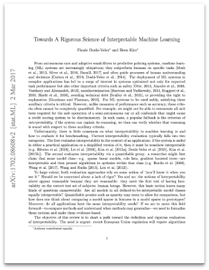
The predicted target \(y\) is a linear combination of the weighted features \(\beta_i x_i\). The estimated linear equation is a hyperplane in the feature/target space (a simple line in the case of a single feature).
The weights specify the slope (gradient) of the hyperplane in each direction.
Linear Regression
![]()
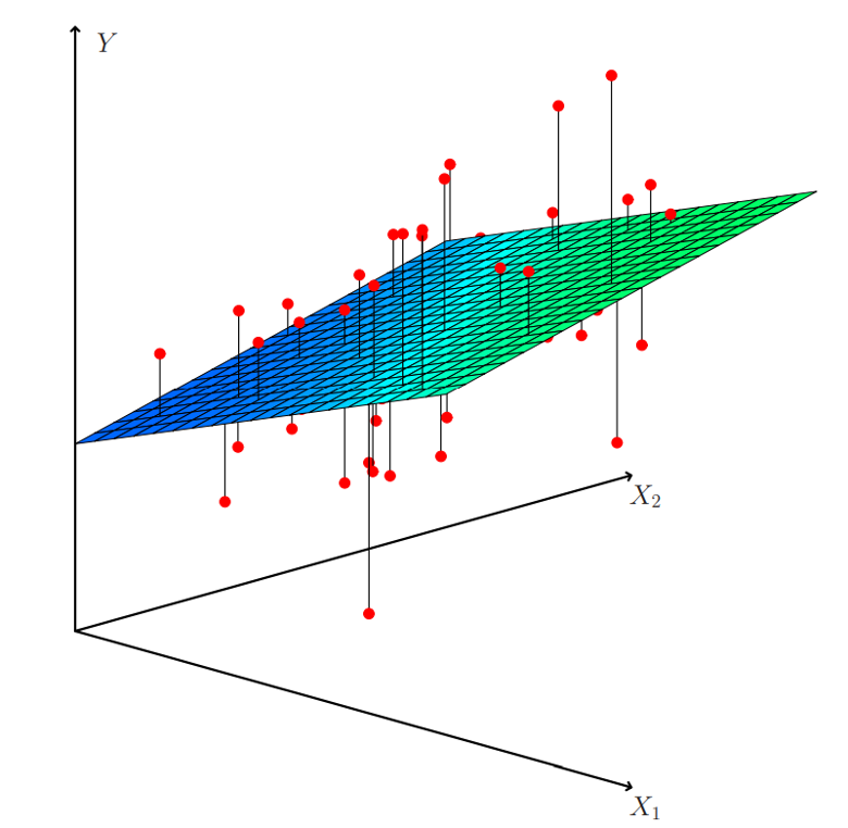
Linear Regression: An Example of Housing Price
![]()
How do you interpret the influence of each property on the prediction of housing price?
Evaluation of Linear Regression Model
R Square
\(R^2\) (R-squared) \[\begin{equation}
R^2 = 1 - \frac{\sum (y_i - \hat{y}_i)^2}{\sum (y_i - \bar{y})^2}
\end{equation}\]
Mean Square Error (MSE)/Root Mean Square Error (RMSE)
\[\begin{equation}
MSE = \frac{1}{N} \sum_{i=1}^{N} (y_i - \hat{y}_i)^2
\end{equation}\]
Mean Absolute Error (MAE)
\[\begin{equation}
MAE = \frac{1}{N} \sum_{i=1}^{N} |y_i - \hat{y}_i|
\end{equation}\]
Visual Analytics (VA) Systems for Linear Regression
There is a trade-off between model complexity (number of features) and accuracy.
This VA system helps model building (feature ranking) and model validation.
Pros and Cons of Linear Models
Pros and Cons of Linear Models
Pros:
Easily interpretable
Statistical guarantees on inference (if assumptions are satisfied)
No hyperparameters (analytical solution)
Cons:
\(X\)’s relationship with \(Y\) can be non-linear. In these cases, linear regression may not provide good results.
If you don’t satisfy certain assumptions (namely normal distribution of residuals and homoscedasticity), then inference can be incorrect.
Limitations of Linear Models
- Features are assumed to follow Gaussian distribution
- No interactions between features
What if your dataset does not follow the assumptions?
Generalized Additive Models (GAMs)
Generalized additive models extend standard linear models by allowing non-linear functions of each of the variables. \[\begin{equation}
y_i = \beta_0 + \sum_{j=1}^{p} f_j(x_{ij}) + \varepsilon_i \\
= \beta_0 + f_1(x_{i1}) + f_2(x_{i2}) + \dots + f_p(x_{ip}) + \varepsilon_i
\end{equation}\]
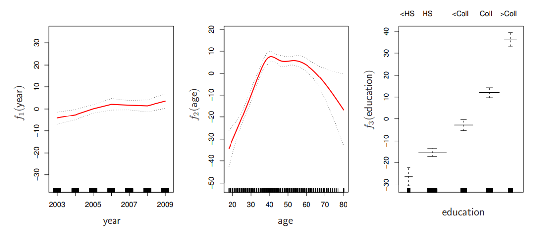
Generalized Additive Models (GAMs): An Example
\[\begin{equation}
Wage = f(year, age, education) = b_0 + f_1(year) + f_2(age) + f_3(education)
\end{equation}\] ![]()
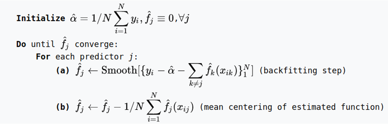
Training GAMs (Backfitting)
![]()
Generalized Additive Models (GAMs): Pros and Cons
Pros:
GAMs allow us to fit a non-linear \(f_j\) to each \(X_j\) , so that we can model non-linear relationships easily.
The non-linear fits can potentially lead to better predictions.
Because the model is additive, we can examine the effect of each \(X_j\) on \(Y\) for each observation. This is useful for visualization.
Cons:
GAMs are restricted to be additive. With many variables, important interactions can be missed or computationally infeasible to find.
Explainable Boosting Machines
\[\begin{equation}
g(\mathbb{E}[y]) = \beta_0 + \sum f_j(x_j)
\end{equation}\]
\[\begin{equation}
g(\mathbb{E}[y]) = \beta_0 + \sum f_j(x_j) + \sum f_{ij}(x_i, x_j)
\end{equation}\]
However, as with linear regression, we can manually add interaction terms to the GAM model by including additional predictors of the form \(X_j \times X_k\). In addition we can add low-dimensional interaction functions of the form \(f_{jk}(X_j , X_k)\) into the model.
Explainable Boosting Machines
\[\begin{equation}
g(\mathbb{E}[y]) = \beta_0 + \sum f_j(x_j)
\end{equation}\]
\[\begin{equation}
g(\mathbb{E}[y]) = \beta_0 + \sum f_j(x_j) + \sum f_{ij}(x_i, x_j)
\end{equation}\]
What if we have a lot of interactions? How do we choose our interactions?
Explainable Boosting Machines
![]()
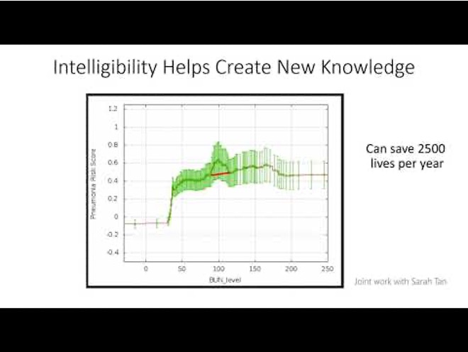
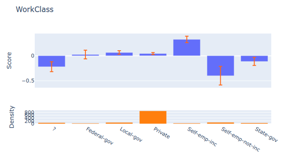
Visualizing EBMs (or GAMs)
![]()
Partial dependency plot
Visualizing EBMs (or GAMs)
![]()
Partial dependency plot
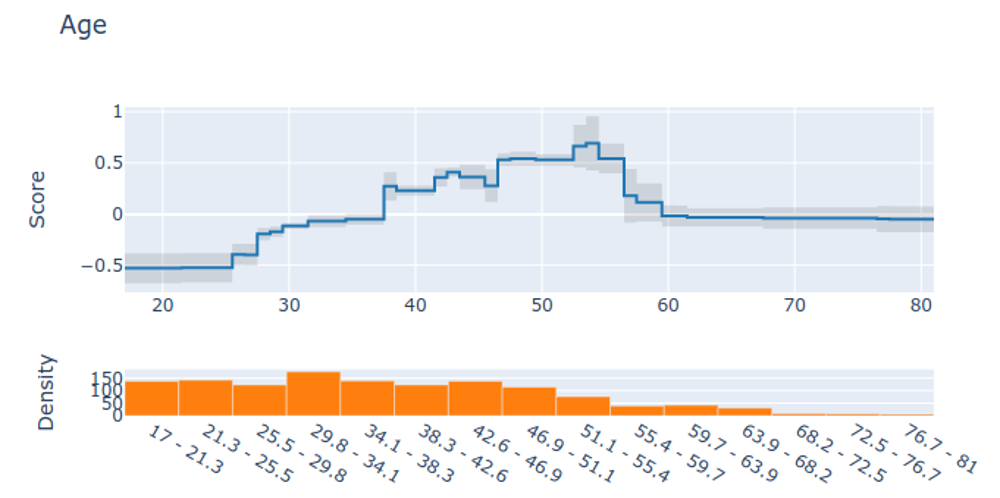
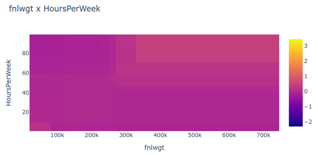
Visualizing EBMs (or GAMs)
![]()
Partial dependency plot
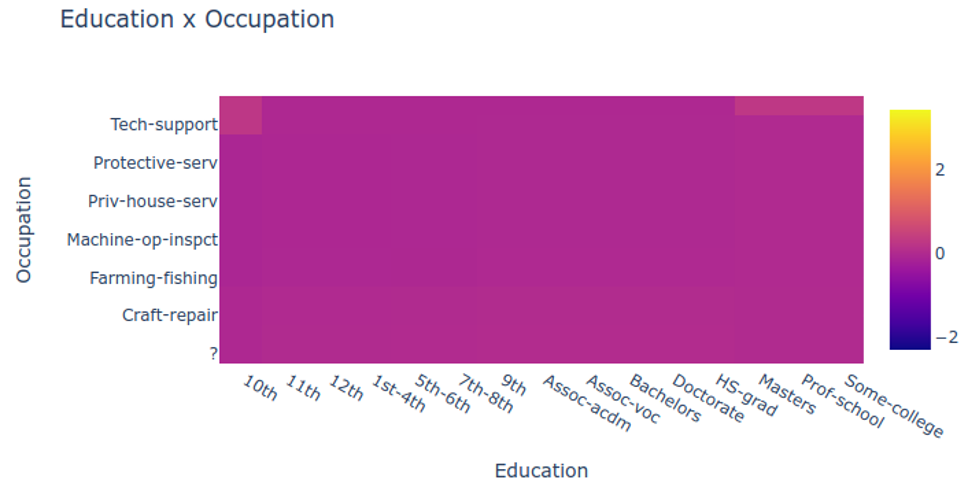
Visualizing EBMs (or GAMs)
![]()
Partial dependency plot
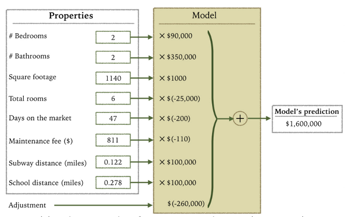
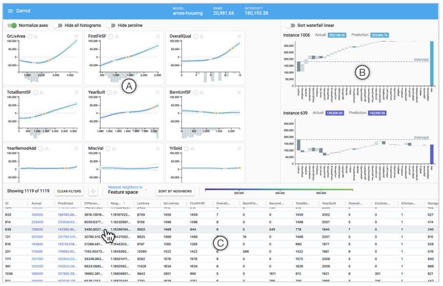
Visual Analytics (VA) Systems Using GAMs
![]()
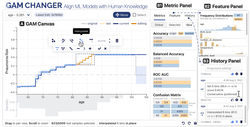
Visual Analytics (VA) Systems Using GAMs
![]()
GAM Changer
https://arxiv.org/pdf/2112.03245.pdf https://github.com/interpretml/gam-changer
Practice 1
Notebook: https://colab.research.google.com/drive/1nKE6WIApebHi67yfhH6k5mZN86evLZOM?usp=sharing
Some other libraries for PDP visualization: https://scikit-learn.org/stable/modules/partial_dependence.html https://interpret.ml/docs/pdp.html
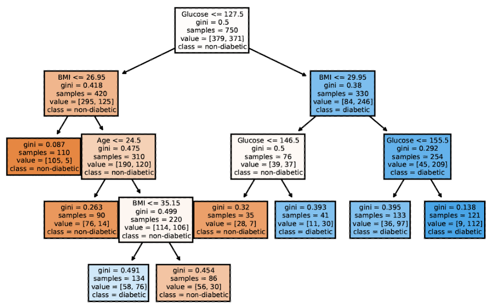
Tree-based Models: Example
![]()
A decision tree of diabetes diagnosis
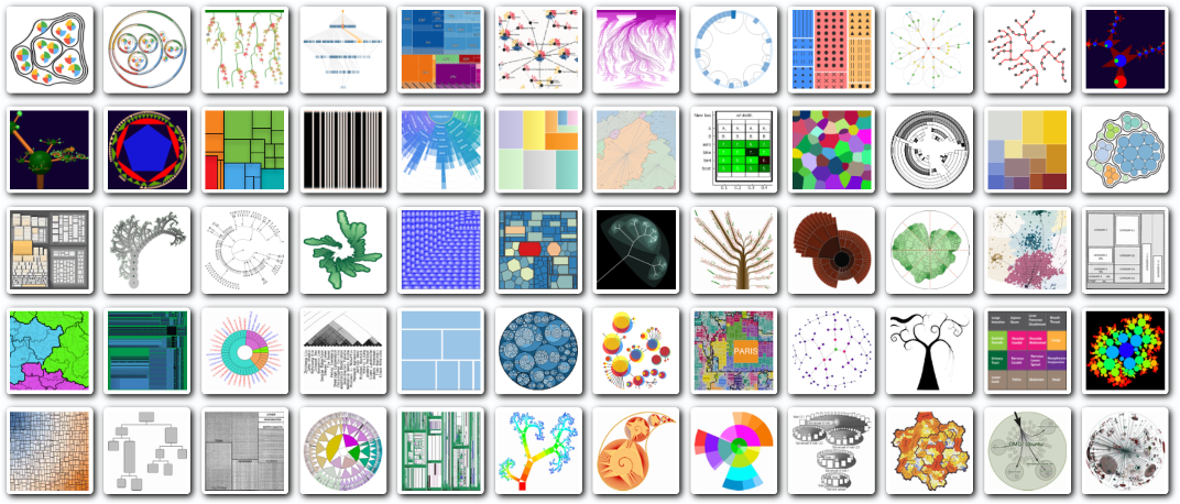
Visualization of Trees
https://treevis.net/ provides a gallery of tree visualization. These trees are used to visualize hierarchical structures, but not just tree-based machine learning models. ![]()
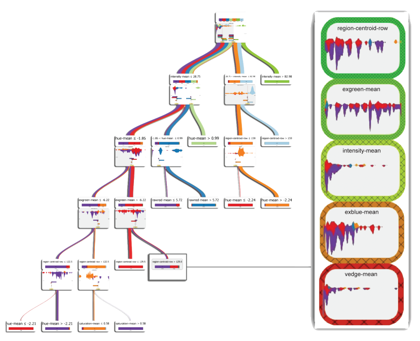
VA Systems Using Tree-based Models
It shows the flow of different class, and the class distribution in along the feature values.
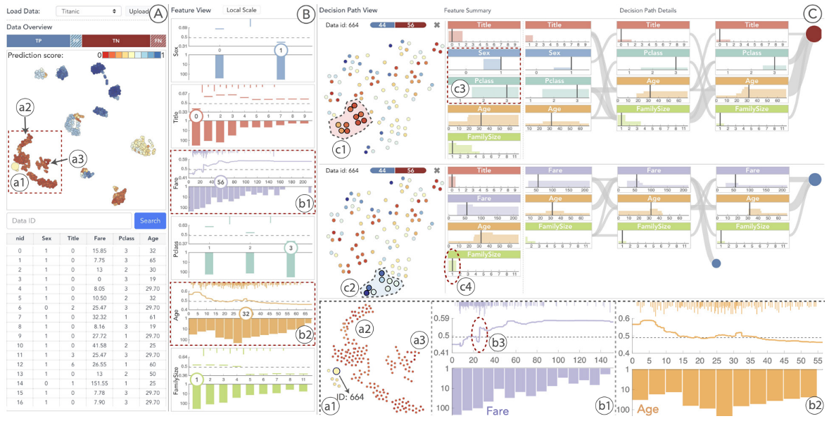
VA Systems Using Tree-based Models
![]()
iForest
Decision Rules: Different Structures
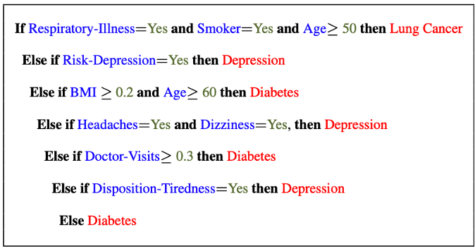
![Rule List: If-then-else structure.]() Clearly see how the decision is made and which rule is more important.
Clearly see how the decision is made and which rule is more important.
The final decision is made based on a voting mechanism.
A recent user study shows that “if-then structure without any connecting else statements enables users to easily reason about the decision boundaries of classes.”
Decision Rules: Different Structures
Disjunctive normal form (DNF, OR-of-ANDs) Conjunctive normal form (CNF, AND-of-ORs)
![]()
What form does this rule set follow?
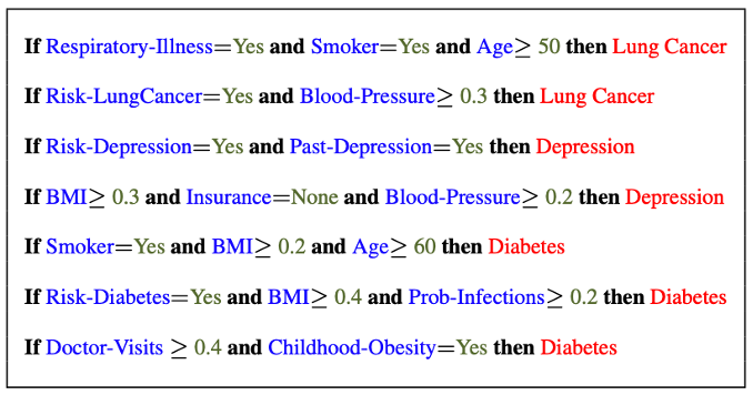
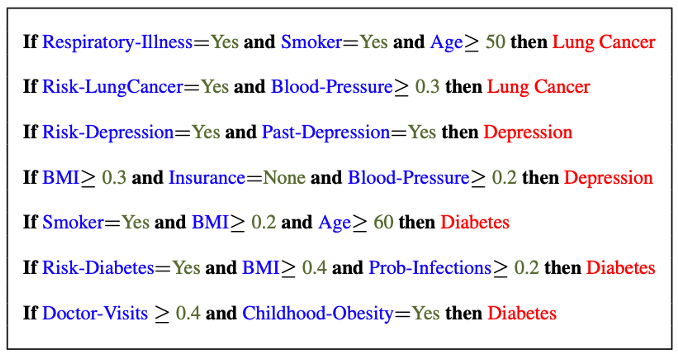
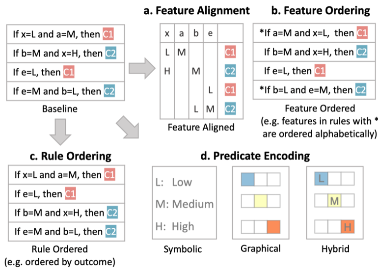
Decision Rules: Visual Factors Influence Rule Understanding
Can different visualizations of rules lead to different level of understanding of rules?
If so, what are the visual factors influence understanding and how they play a role in rule understanding?
Evaluation of Rules
Given a rule below:
If \(X\), then class \(Y\).
Support / Coverage of a rule:
\[\begin{equation}
\text{Support} = \frac{\text{number of instances that match the conditions in } X}{\text{total number of instances}}
\end{equation}\]
Confidence / Accuracy of a rule:
\[\begin{equation}
\text{Confidence} = \frac{\text{number of instances that match conditions in } X \text{ and belong to class } Y}{\text{number of instances that match conditions in } X}
\end{equation}\]
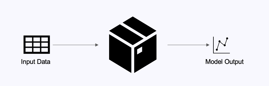
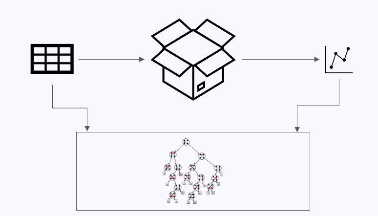
Global Surrogate
Imagine that we have a black-box model (too complex to understand the internal structure), can we use white-box models to help us understand the model behavior of the black-box model? ![]()
Global Surrogate
Open the black box by understanding a “surrogate model” that approximate the behavior of the original black-box model. ![]()
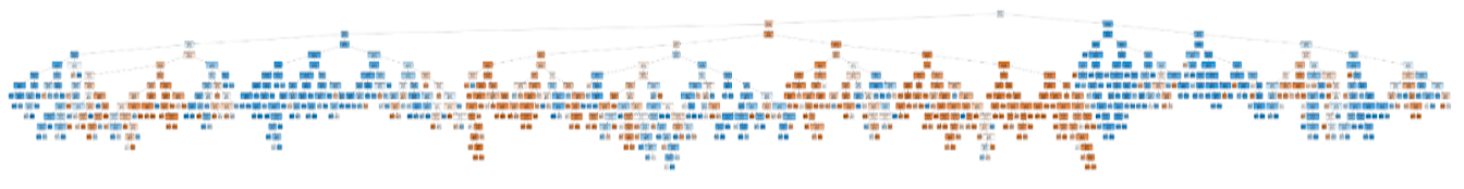
However…
What you want:
![]()
What you get:
![]()
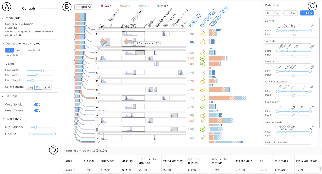
VA System for Rule List
![]()
RuleMatrix
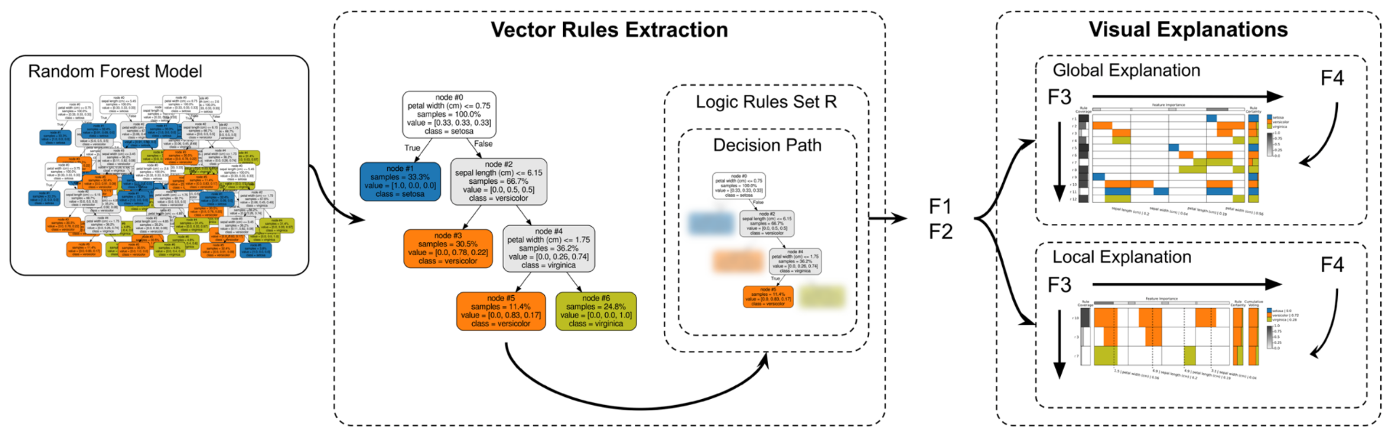
VA Systems for Rules in Random Forest
![]()
Explainable Matrix
Other white-box models?
- Naive Bayes
- K-nearest neighbors
- etc.
Practice 2
Notebook: https://colab.research.google.com/drive/12LV2Z_1BbP3efACYp2QxzsPaOrIn8a8l?usp=sharing
Today’s Class
- Model Interpretation and Explanation
- White-box Approaches and Visualizations
- Related Research in VIS & AI
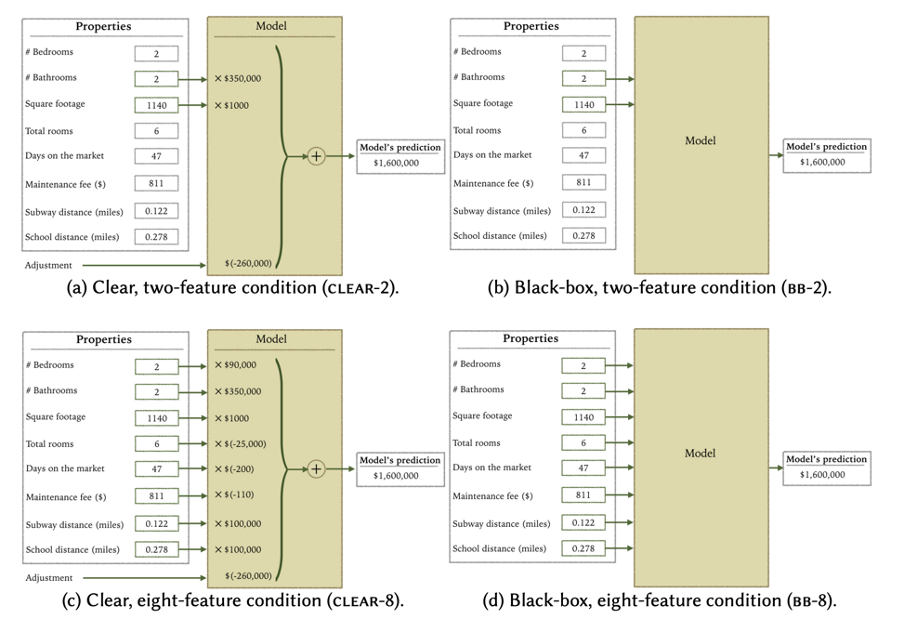
Manipulating and Measuring Model Interpretability
![]()
https://arxiv.org/abs/1802.07810
Stop explaining black box machine learning models for high stakes decisions
![]()
https://www.nature.com/articles/s42256-019-0048-x
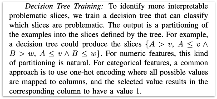
Slice Finder: Automated Data Slicing for Model Validation
How about we use whether the model prediction is wrong or not to train a “surrogate tree”?
https://ieeexplore.ieee.org/stamp/stamp.jsp?tp=&arnumber=8731353


 Clearly see how the decision is made and which rule is more important.