Week 10 Lab: 3D Visualization: Transformations
CS-GY 6313 - Information Visualization
Ryan Kim
New York University
2025-11-07
Week 9 Lab Overview
Today’s Lab Activities
Today we will be a exploring the following topics:
- Group and Mini Projects: Reminders
- Main Lab Activities:
- Common Libraries for 3D Visualizations
- Re-Visiting Algebra
- 2D Transformations
- Homogeneous Coordinates
- 3D Transformations
- Model-View-Projection
Group and Mini Projects: Reminders
| Milestone #3: First Draft |
Nov. 17 |
Initial D3 implementations |
| Mini-Project #2 |
Nov. 20 |
Temporal Data Visualizations |
Group Project Milestone #3: Deliverables
Submit an Observable notebook or a Framework project with:
- Brief introduction to your project
- For each question:
- State the question
- Show the D3 visualization
- Describe what the visualization shows
- Answer the question based on the visualization
At this stage:
- All visualizations should be implemented in D3
- Focus on getting the basics working
- Styling/polish can come later
- Interactivity should be functional (if included)
- It’s still okay to refine questions if needed
Group Project Milestone #3: Reminders
This is your first implementation milestone.
- We expect working D3 code for all your visualizations.
- Your visualizations don’t need to be perfect, but they should work and show your data correctly.
- labels might be messy
- colors might be defaults
- interactions might be basic
- This is when you discover implementation challenges:
- “This chart type is harder than I thought…”
- “The data is more complex than I realized…”
- We’ll give you feedback on what to improve for the next draft.
Common Libraries for 3D Visualization
How Do These Libraries Work?
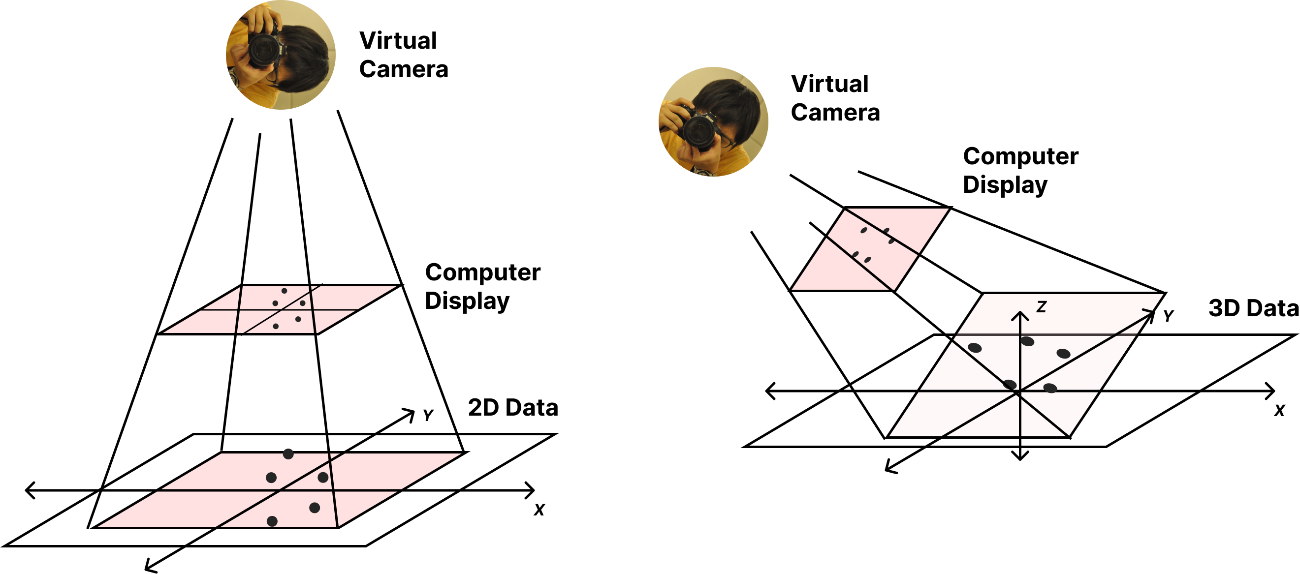
Our data resides within a 2D or 3D space, as viewed by the user through a 2D viewpoint. How the data is projected onto the screen, relative to the viewpoint, is a fundamental operation in most 2D and 3D graphics libraries.
![]()
How Do These Libraries Work?
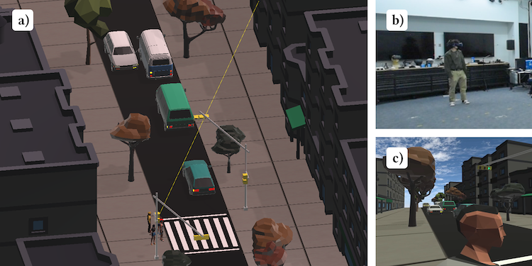
These fundamental operations are crucial in other domains beyond just data visualization, such as video games, virtual reality, interactive computer graphics, and 3D CAD tools.
![]()
Ryan Kim and Paul M. Torrens. 2024. Building Verisimilitude in VR With High-Fidelity Local Action Models: A Demonstration Supporting Road-Crossing Experiments. In 38th ACM SIGSIM Conference on Principles of Advanced Discrete Simulation (SIGSIM PADS ’24), June 24–26, 2024, Atlanta, GA, USA. ACM, New York, NY, USA, 12 pages. https://doi.org/10.1145/3615979.3656060
Revisiting Algebra: Vectors
Vectors
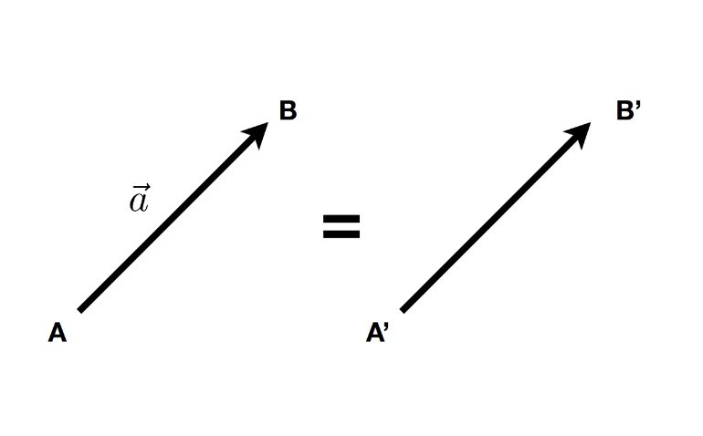
- A vector \(\overrightarrow{(x, y, z, …)}\) describes a direction and a length without a starting point.
- A vector is NOT a pair \({x,y}\), NOR a position \((x,y)\)
\[
\overrightarrow{AB} = B - A
\]
- A unit vector is a vector with length = 1 (direction-only)
\[
\hat{a} = \frac{\overrightarrow{a}}{\|\overrightarrow{a}\|}
\]
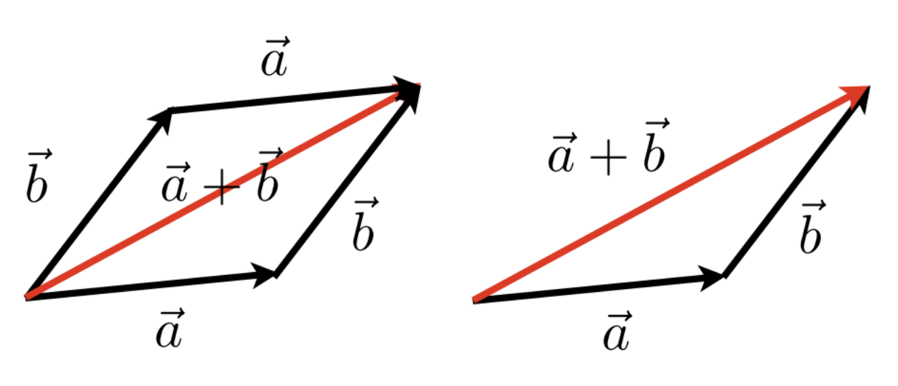
Vector Math
\[
\overrightarrow{a} + \overrightarrow{b} = \overrightarrow{b} + \overrightarrow{a}
\]
Dot Product
\[
\overrightarrow{a} \cdot \overrightarrow{b} = \|\overrightarrow{a}\|\|\overrightarrow{b}\|\cos{\theta}
\]
\[
\cos{\theta} = \frac{\overrightarrow{a} \cdot \overrightarrow{b}}{\|\overrightarrow{a}\|\|\overrightarrow{b}\|}
\]
Cross Product
- Orthogonal to two initial vectors
- Direction determined by right-hand rule
- Useful in constructing coordinate systems
Revisiting Algebra: Matrices
\[
\begin{pmatrix} 1 & 2 & 3 \\ 4 & 5 & 6 \end{pmatrix}
\]
- Matrix: An array of numbers, with \(N\) rows and \(M\) columns.
Multiplication
- Imagine you want to multiply two matrices: \(A\) (an \(N \times M\) matrix) and \(B\) (an \(M \times P\) matrix) …
- The number of columns in A must MUST = the number rows in B.
- The outcome = an \((M \times P)\) matrix
- \((M \times N) (N \times P) = (M \times P)\)
\[
\begin{pmatrix}a & b \\ c & d\end{pmatrix} \begin{pmatrix}e & f \\ g & h\end{pmatrix} = \begin{pmatrix} ae + bg & af + bh \\ ce + dg & cf + dh \end{pmatrix}
\]
Let’s Practice
\[
\begin{pmatrix} 1 & 3 \\ 5 & 2 \\ 0 & 4 \end{pmatrix}\begin{pmatrix}3 & 6 & 9 & 4 \\ 2 & 7 & 8 & 3 \end{pmatrix} = \begin{pmatrix}9 & ? & 33 & 13 \\ 19 & 44 & 61 & 26 \\ 8 & 28 & 32 & ? \end{pmatrix}
\]
Keep in Mind:
- Keep in mind that matrix multiplication is:
- Non-commutative (AB and BA are different in general)
- Associative and distributive
- \(A(B+C) = AB + AC\)
- \((A+B)C = AC + BC\)
Matrix-Vector Multiplication
- Treat vector as a column matrix \((m \times 1)\)
\[
\begin{pmatrix}-1 & 0 \\ 0 & 1\end{pmatrix}\begin{pmatrix}x \\ y\end{pmatrix} = \begin{pmatrix}-x \\ y\end{pmatrix}
\]
Transformations: Scaling
![]()
\[
\begin{bmatrix}x' \\ y'\end{bmatrix} = \begin{bmatrix}s & 0 \\ 0 & s\end{bmatrix}\begin{bmatrix}x \\ y\end{bmatrix}
\]
Transformations: Scaling
![]()
\[
\begin{bmatrix}x' \\ y'\end{bmatrix} = \begin{bmatrix}s_x & 0 \\ 0 & s_y\end{bmatrix}\begin{bmatrix}x \\ y\end{bmatrix}
\]
Transformations: Reflection
![]()
\[
\begin{bmatrix}x' \\ y'\end{bmatrix} = \begin{bmatrix}s_x & 0 \\ 0 & s_y\end{bmatrix}\begin{bmatrix}x \\ y\end{bmatrix}
\]
Transformations: Reflection
![]()
\[
\begin{bmatrix}x' \\ y'\end{bmatrix} = \begin{bmatrix}-1 & 0 \\ 0 & 1\end{bmatrix}\begin{bmatrix}x \\ y\end{bmatrix}
\]
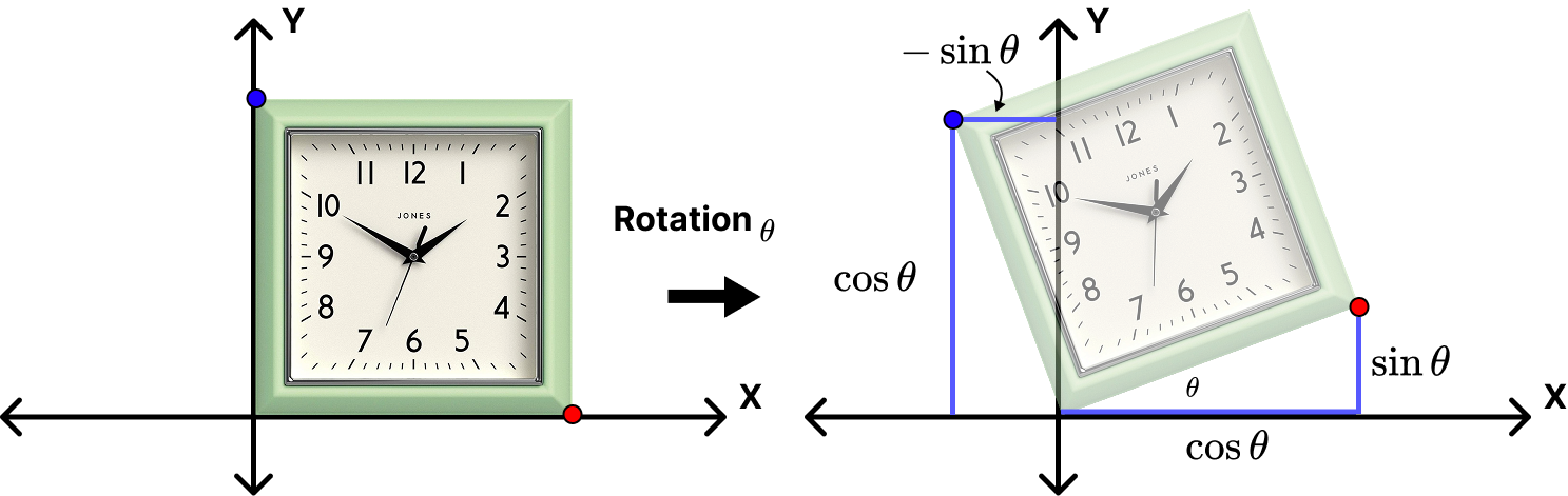
Transformations: Rotation
![]()
\[
R_\theta = \begin{bmatrix}\cos{\theta} & -\sin{\theta} \\ \sin{\theta} & \cos{\theta} \end{bmatrix}
\]
Transformations: The Pattern
\[
\begin{bmatrix}x' \\ y'\end{bmatrix} = \begin{bmatrix}a & b \\ c & d\end{bmatrix}\begin{bmatrix}x \\ y\end{bmatrix}
\]
\[
x' = Mx
\]
We generally try to minimize transformation operations by relying on single transformation matrix \(M\).
Multi-Step Operations
We can perform multiple transformations (e.g. rotation, then scale) in sequence by using multiple \(M\) matrices in sequence. Matrix multiplications occur from right to left and are non-commutative!
\[
\begin{bmatrix}x' \\ y'\end{bmatrix} = \begin{bmatrix}a & b \\ c & d\end{bmatrix} \begin{bmatrix}e & f \\ g & h \end{bmatrix} \begin{bmatrix}x \\ y\end{bmatrix}
\]
\[
x' = M_2M_1x
\]
Transformations: Translations
![]()
\[
\begin{bmatrix}x' \\ y'\end{bmatrix} =\begin{bmatrix}x \\ y\end{bmatrix} + \begin{bmatrix} t_x \\ t_y \end{bmatrix}
\]
Translations Don’t Match the Pattern
- Translation cannot be represented in matrix form
\[
\begin{bmatrix}x' \\ y'\end{bmatrix} = \begin{bmatrix}a & b \\ c & d\end{bmatrix} \begin{bmatrix}x \\ y\end{bmatrix} + \begin{bmatrix} t_x \\ t_y \end{bmatrix}
\]
- Is there a unified way to represent all transformations?
Solution: Homogeneous Coordinates
- Add a 3rd coordinate (a \(w\)-coordinate)
- 2D Point: \(\begin{bmatrix}x \\ y \\ 1 \end{bmatrix}\)
- 2D Vector: \(\begin{bmatrix}x \\ y \\ 0 \end{bmatrix}\)
- Matrix Operations now in Linear Form
\[
\begin{bmatrix}x' \\ y' \\ w' \end{bmatrix} = \begin{bmatrix} 1 & 0 & t_x \\ 0 & 1 & t_y \\ 0 & 0 & 1 \end{bmatrix} \begin{bmatrix}x \\ y \\ 1 \end{bmatrix} = \begin{bmatrix} x + t_x \\ y + t_y \\ 1 \end{bmatrix}
\]
2D Transformations
Scale
\[
S(s_x,s_y)=\begin{bmatrix}
s_x & 0 & 0 \\
0 & s_y & 0 \\
0 & 0 & 1 \end{bmatrix}
\]
Rotation
\[
R(\theta)=\begin{bmatrix}
\cos{\theta} & -\sin{\theta} & 0 \\
\sin{\theta} & \cos{\theta} & 0 \\
0 & 0 & 1 \end{bmatrix}
\]
Translation
\[
T(t_x,t_y)=\begin{bmatrix}
1 & 0 & t_x \\
0 & 1 & t_y \\
0 & 0 & 1 \end{bmatrix}
\]
3D Transformations
We do the same thing that we did with 2D matrices: add another column! This also means that transformations using homogeneous coordinates involves \(4 \times 4\) matrices.
- 3D point: \((x, y, z, 1)^T\)
- 3D vector: \((x, y, z, 0)^T\)
\[
\begin{bmatrix} x' \\ y' \\ z' \\ 1 \end{bmatrix} = \begin{bmatrix} a & b & c & t_x \\ d & e & f & t_y \\ g & h & i & t_z \\ 0 & 0 & 0 & 1 \end{bmatrix} \begin{bmatrix} x \\ y \\ z \\ 1 \end{bmatrix}
\]
3D Transformations: Scale and Translation
Scale
\[
S(s_x,s_y,s_z) = \begin{bmatrix} x' \\ y' \\ z' \\ 1 \end{bmatrix} = \begin{bmatrix} s_x & 0 & 0 & 0 \\ 0 & s_y & 0 & 0 \\ 0 & 0 & s_z & 0 \\ 0 & 0 & 0 & 1 \end{bmatrix}
\]
Translation
\[
S(s_x,s_y,s_z) = \begin{bmatrix} x' \\ y' \\ z' \\ 1 \end{bmatrix} = \begin{bmatrix} 0 & 0 & 0 & t_x \\ 0 & 0 & 0 & t_y \\ 0 & 0 & 0 & t_z \\ 0 & 0 & 0 & 1 \end{bmatrix}
\]
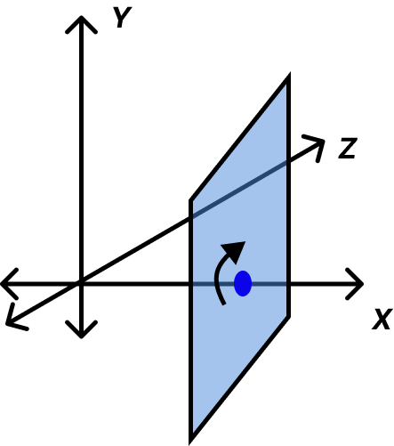
3D Transformations: Rotations
We need to consider 3 axes rather than just a singular axis like in 2D…
\[
R_x(\theta) = \begin{bmatrix} 1 & 0 & 0 & 0 \\ 0 & \cos{\theta} & -\sin{\theta} & 0 \\ 0 & \sin{\theta} & \cos{\theta} & 0 \\ 0 & 0 & 0 & 1 \end{bmatrix}
\]
\[
R_y(\theta) = \begin{bmatrix} \cos{\theta} & 0 & \sin{\theta} & 0 \\ 0 & 1 & 0 & 0 \\ -\sin{\theta} & 0 & \cos{\theta} & 0 \\ 0 & 0 & 0 & 1 \end{bmatrix}
\]
\[
R_z(\theta) = \begin{bmatrix} \cos{\theta} & -\sin{\theta} & 0 & 0 \\ \sin{\theta} & \cos{\theta} & 0 & 0 \\ 0 & 0 & 1 & 0 \\ 0 & 0 & 0 & 1 \end{bmatrix}
\]
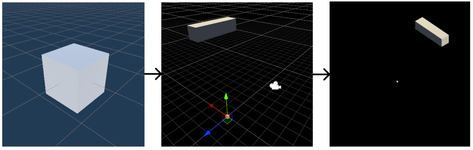
Applications: Model-View-Projection
At its core, the task of rendering 3D data requires a kind of “pipeline” - a series of transformations from one “space” to another, in sequence:
| Data points are placed within the 3D “world”. |
All points are transformed and are now relative to the camera’s space. |
All points are projected onto the 2D screen. |
![]()
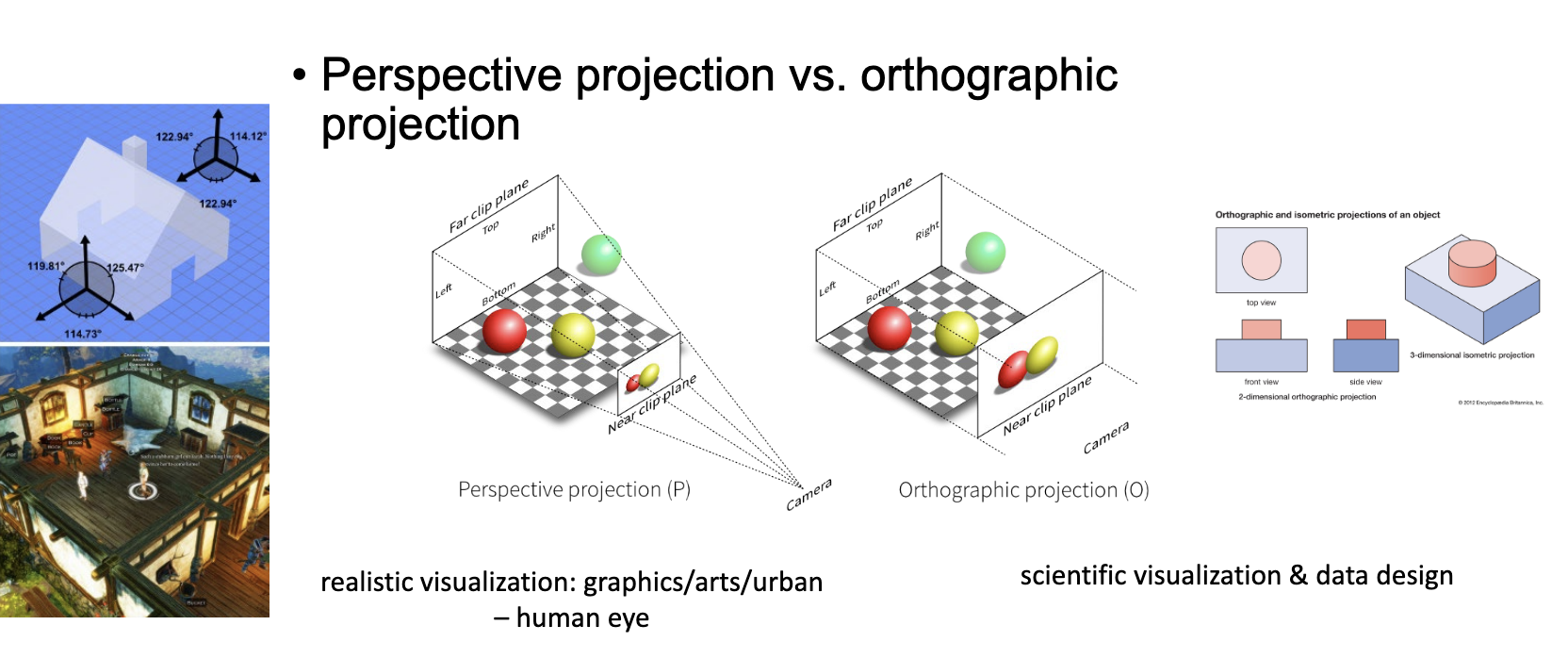
Model-View-Projection Transformations
- Find a good place to stand (model transformation)
- Find a good “angle” to place the camera (view transformation)
- Cheeese! (projection transformation)
This MODEL-VIEW-PROJECTION operation is instrumental to all graphics libraries, render engines, etc.
![]()