What’s the difference between data and information?
Food 4 Thought: “Data” v.s. “Information”
A Question:
What’s the difference between data and information?
Data v.s. Information
Data:
Facts and statistics collected together for reference or analysis. Can be structured/unstructured, quantitative/qualitative, temporal/static.
E.g. Census data, stock prices, sensor readings, survey responses, click streams.
Alone, it lacks context and meaning.
Information:
Processed and/or organized form of data.
E.g. Sales reports, news articles, graphs & figures.
Analyzed, structured, and given context through a narrative established by its handlers.
Meaning-Making: Data -> Information
As engineers, designers, and researchers, we must do the work to find meaning within the raw data and interpret them for the benefit of others.
Dataset: Movies
Vega-Lite contains several datasets available to us. We’ll be using a dataset that describes movies.
movies = (awaitrequire('vega-datasets@1'))['movies.json']()
Features/Columns:
Title
US_Gross
Worldwide_Gross
US_DVD_Sales
Production_Budget
Release_Date
MPAA_Rating
Running_Time_min
Distributor
Source
Major_Genre
Creative_Type
Director
Rotten_Tomatoes_Rating
IMDB_Rating
IMDB_Votes
Review: 4 Major Data Transformations
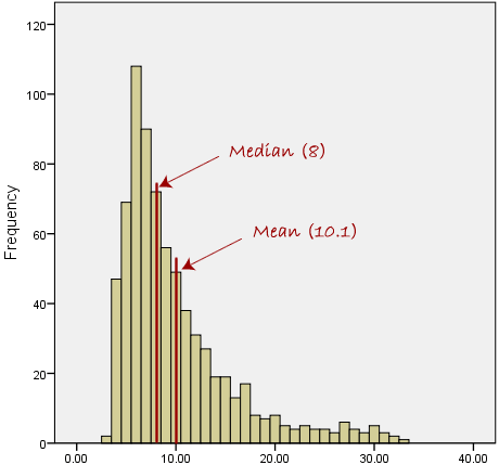
Aggregation
Purpose: Summarize groups of data
Methods: Sum, mean, median, count, min, max
Example: Daily sales → Monthly totals
Filtering
Purpose: Focus on relevant subset
Types: Range, categorical, conditional
Binning
Purpose: Convert continuous to discrete
Methods: Equal width, equal frequency, custom _ Example: Dividing age into groups (<18, 18-65, >65)
Normalization
Purpose: Enable fair comparison
Methods: Min-max, z-score, percentage
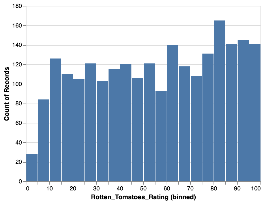
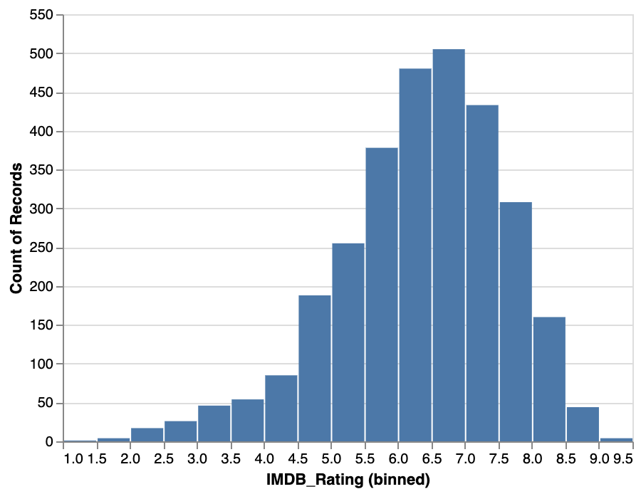
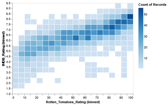
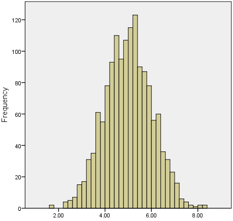
Step 1: Binning
Grouping continuous data into discrete groups.
What are some common examples?
Age groups
NYC Boroughs
Years
Grades/Scores
Any kind of continuous data can be binned, in theory.
We lose a bit of data in the meantime, but by doing so we increase the probability of deriving new meaning.
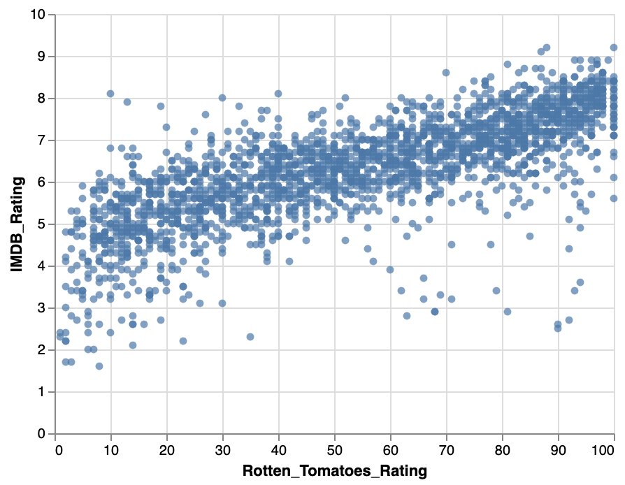
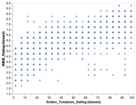
Rotten Tomatoes v.s. IMDb Ratings
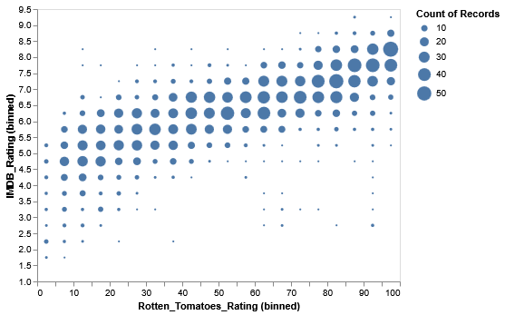
To better understand the importance of aggregation, let’s look at raw, unaggregated data of movie ratings across Rotten Tomatoes and IMDb. We’ll use Vega-Lite to produce a scatter plot using the circle mark.
[TO-DO]: Generate a scatter plot with the circle marker, with the X-axis representing the Rotten Tomatoes ratings (Rotten_Tomatoes_Rating) and IMDb ratings (IMDB_Rating).
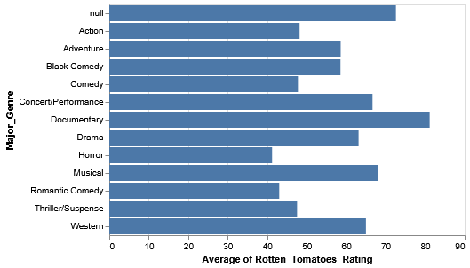
There may be some interesting variation, but it’s mentally tasking to try to understand overall rankings across genres.
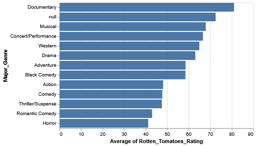
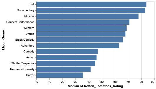
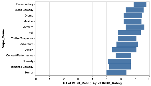
Sorting
Rather than sort the genres alphabetically, let’s try to sort them in descending order of rating (i.e. the genres with the higher ratings are at the top, while the genres with the lower ratings are at the bottom).
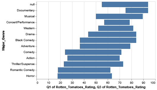
Even with this data, we should still be a bit skeptical. What if, within the genres themselves, there’s some skew caused by outliers and such? Observing the variation within each genre is a good way to extend our analysis.
The IQR is a special range across a set of values that represents where the middle half of the data resides in. A quartile represents 25% of data values. The IQR therefore represents the two middle quartiles, or the middle 50% of data.