Clustering and Dimensionality Reduction

CS-GY 6313 - Fall 2025
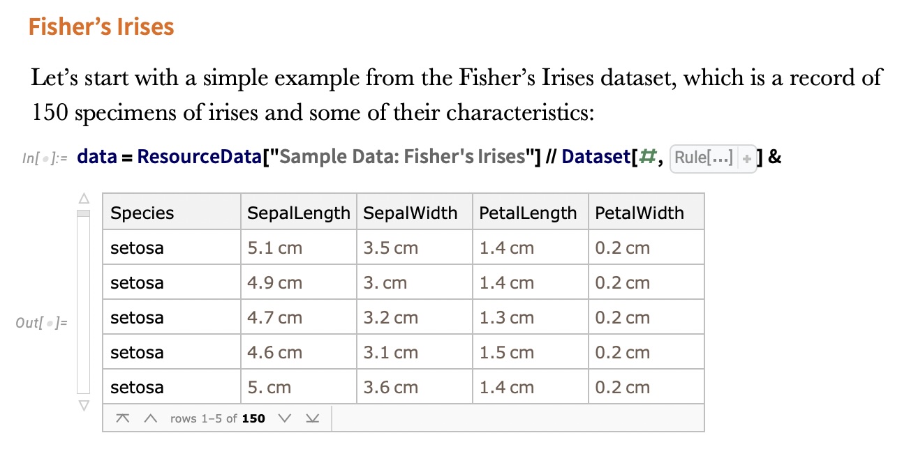
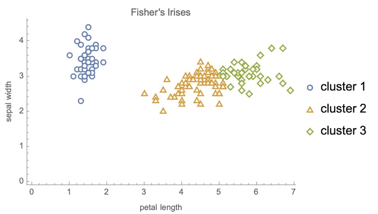
Claudio Silva

Agenda

  1. Clustering Visualization
    • Introduction to clustering analysis
    • K-means and visual patterns
    • Comparing clustering methods
  2. Dimensionality Reduction for Visualization
    • Why reduce dimensions?
    • Linear methods: PCA
    • Non-linear methods: t-SNE and UMAP
    • Critical visualization principles

Clustering Visualization

What is Clustering?

“… the goal of clustering is to separate a set of examples into groups called clusters”

Visualizing the IRIS Dataset

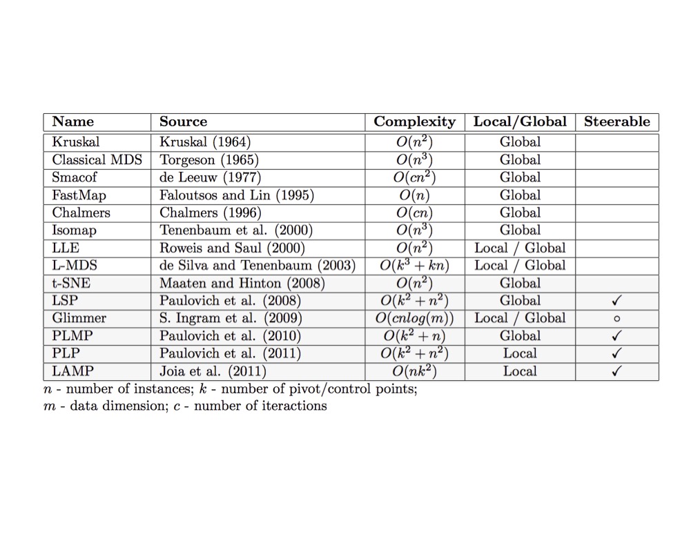
Clustering Methods Comparison
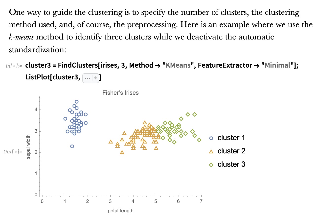
K-means Clustering

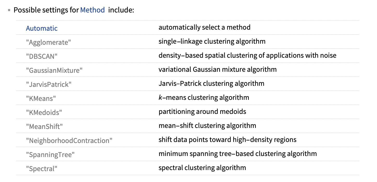
Clustering Method Zoo

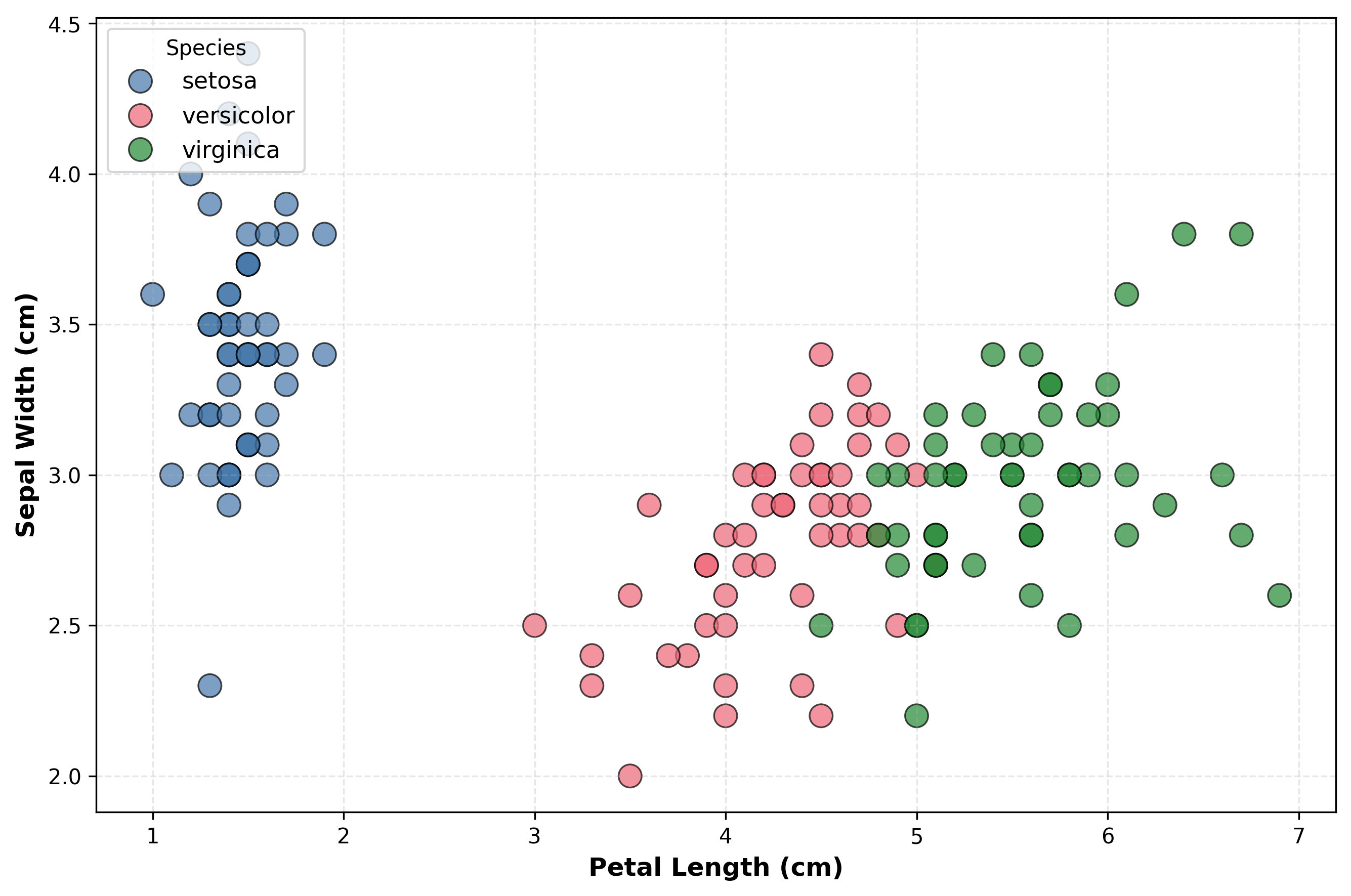
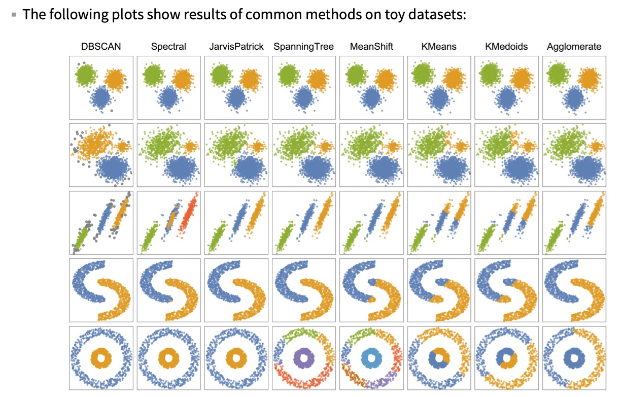
Visual Comparison of Methods

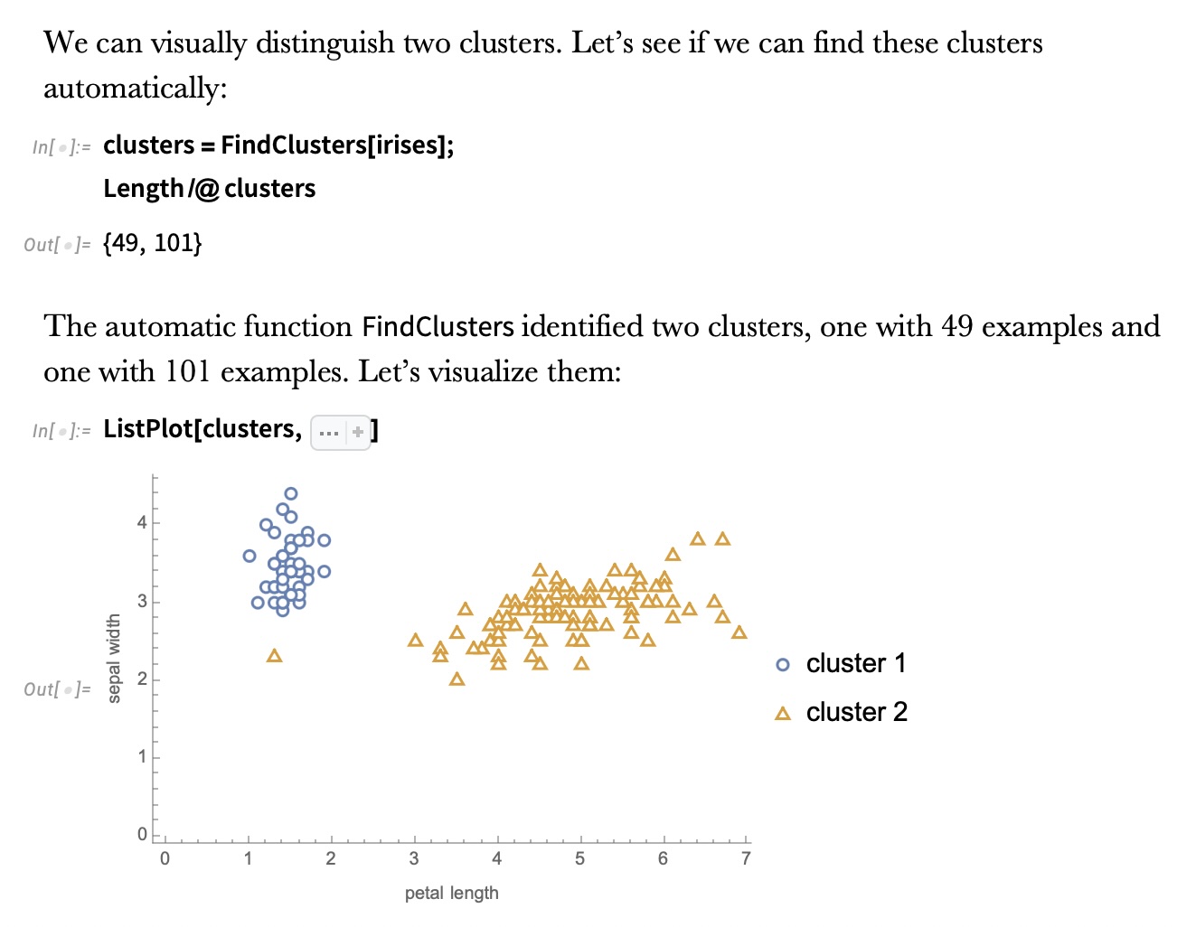
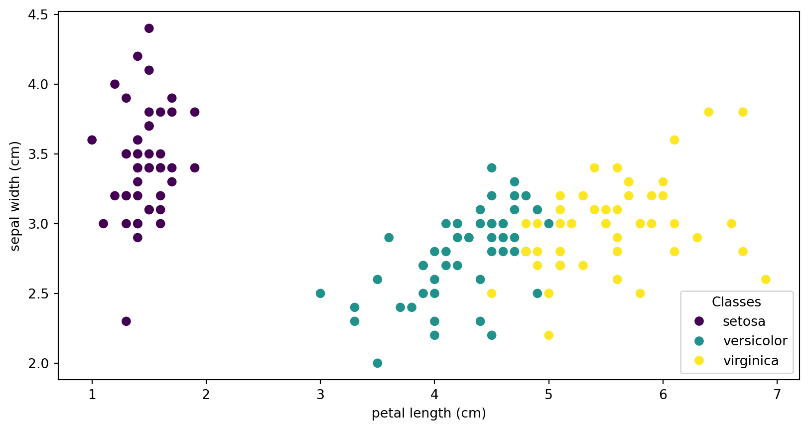
Ground Truth vs K-means

Dimensionality Reduction

The Challenge: High-Dimensional Data

  • Real-world data often has hundreds or thousands of dimensions
    • Images: thousands of pixels
    • Text: thousands of words
    • Urban sensors: hundreds of measurements
    • Customer data: dozens to hundreds of features
  • Problem: We can only visualize 2D or 3D!

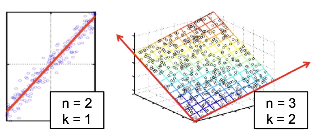
The Manifold Hypothesis

  • Key insight: High-dimensional data often lies on lower-dimensional structures

Non-linear Manifolds

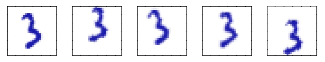
  • Images of ‘3’ transformed by rotation, scaling, translation
  • What’s the intrinsic dimensionality? (~5-7 dimensions)
  • The underlying manifold is non-linear

Working Example: Digits Dataset

from sklearn.datasets import load_digits

digits = load_digits(n_class=6)
X, y = digits.data, digits.target
  • 8×8 pixel images = 64 dimensions
  • Can’t visualize 64D directly
  • Goal: Create meaningful 2D visualization

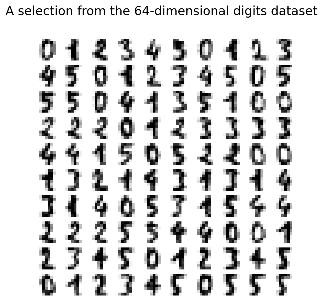
Digits Dataset Sample

Principal Component Analysis (PCA)

PCA: The Foundation

  • PCA finds directions of maximum variance in data
  • These directions are the eigenvectors of the covariance matrix
  • Projects data onto these principal directions
  • Linear method - assumes linear relationships

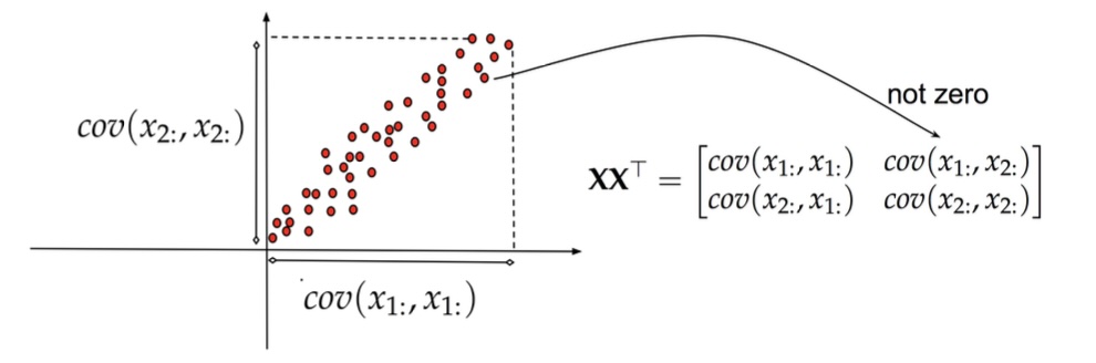
PCA: Geometric Intuition
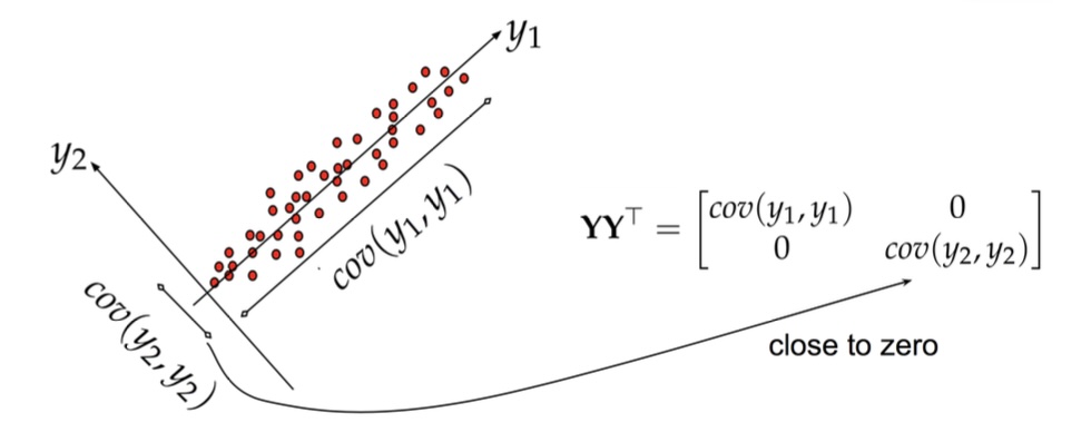
PCA: Another View

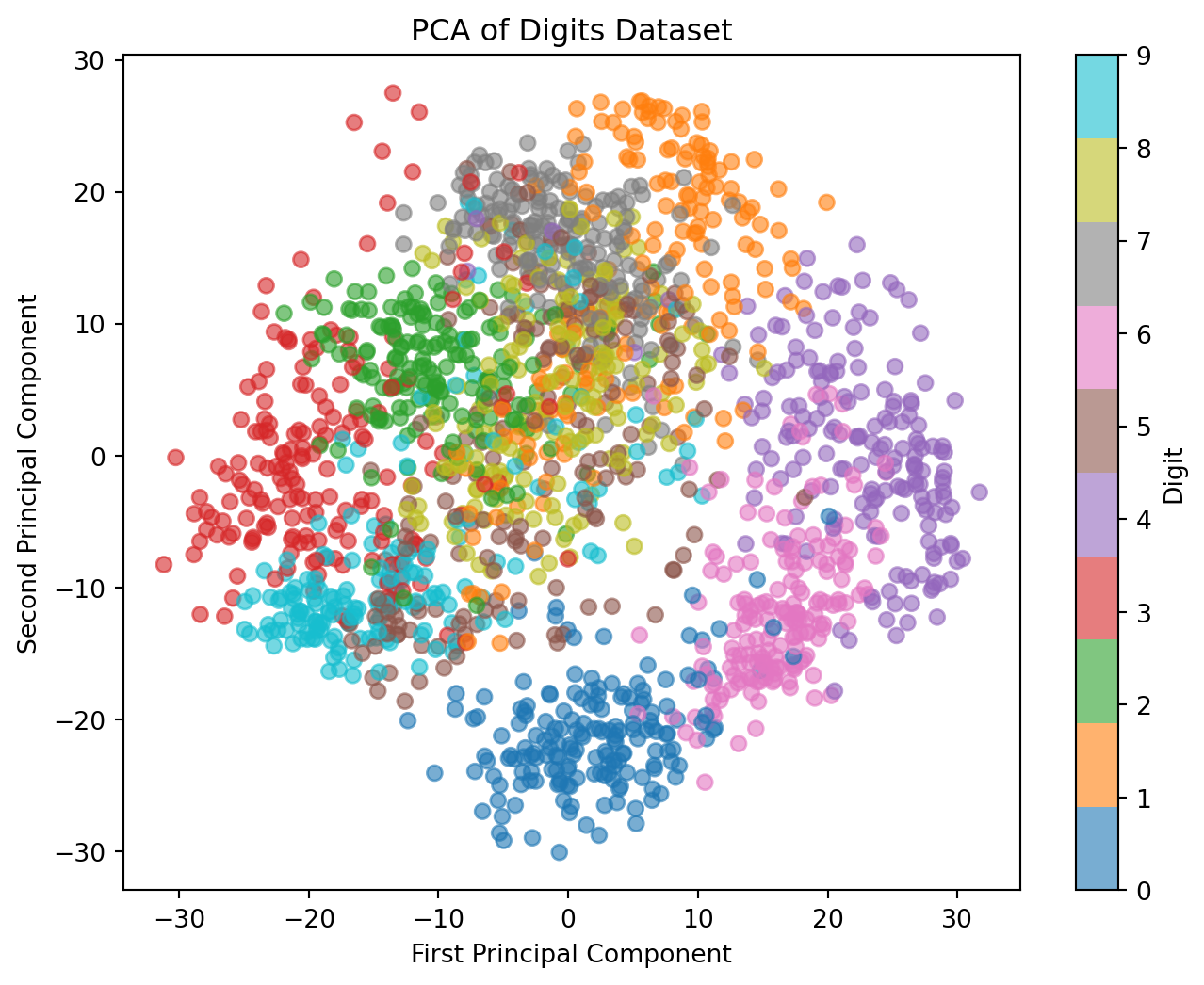
PCA Applied to Digits
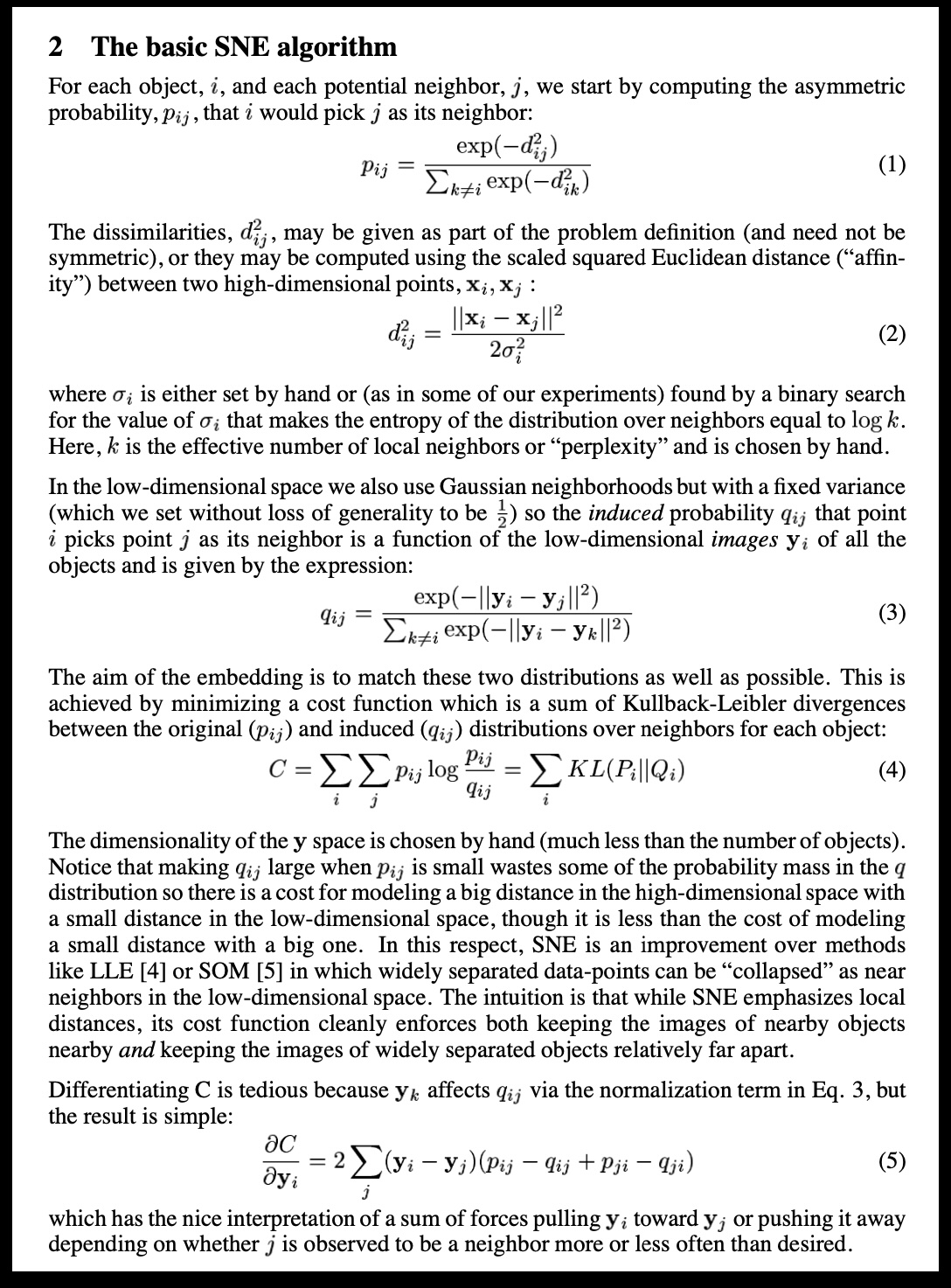
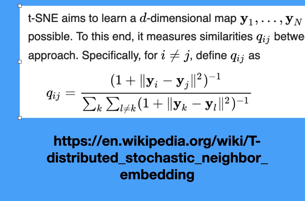
Non-linear Methods: t-SNE

t-SNE: A Revolution in Visualization

  • t-SNE (t-Distributed Stochastic Neighbor Embedding)
    • Preserves local neighborhood structure
    • Non-linear, adapts to different regions of data
    • Creates compelling cluster visualizations
    • Warning: Can be easily misread!

How t-SNE Works

Critical Resource: “How to Use t-SNE Effectively”

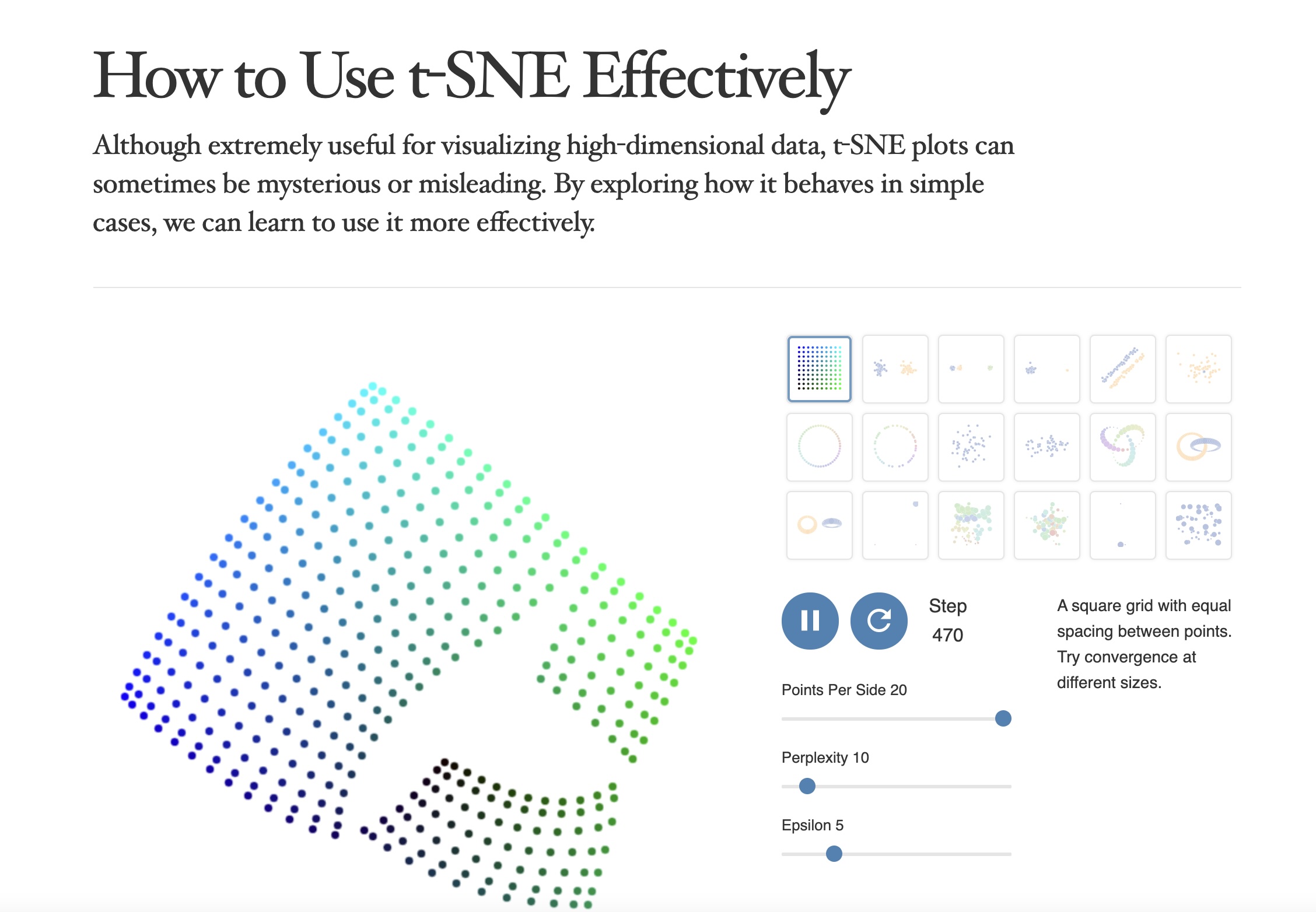
https://distill.pub/2016/misread-tsne/

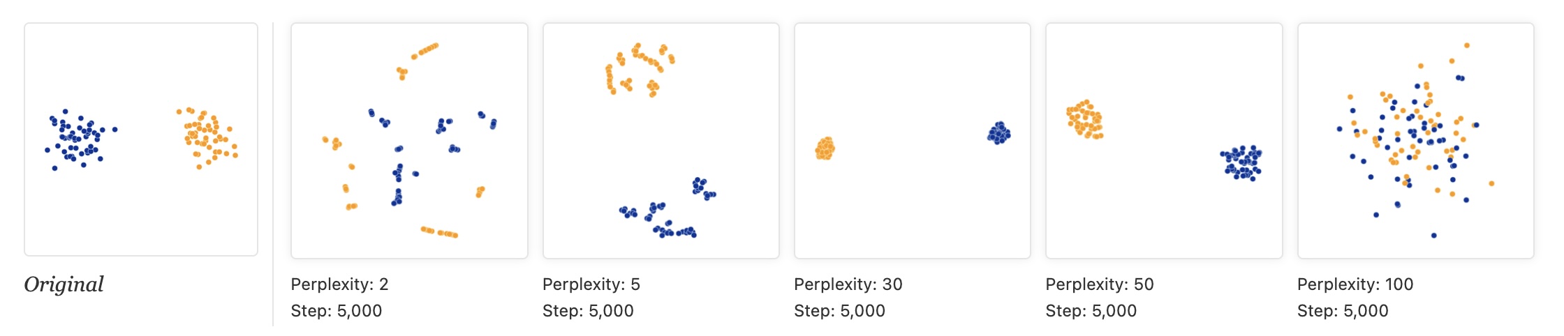
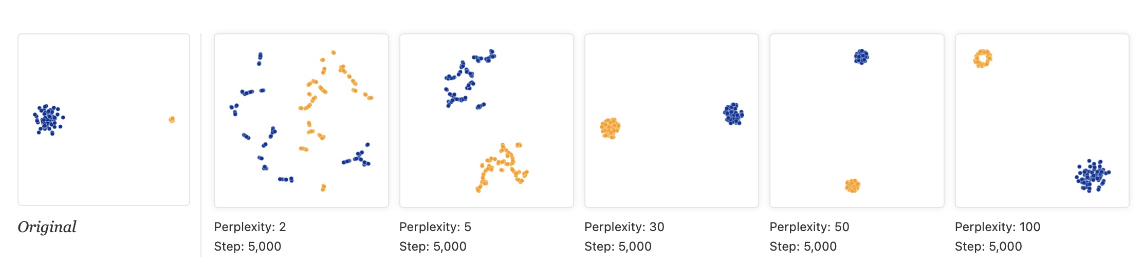
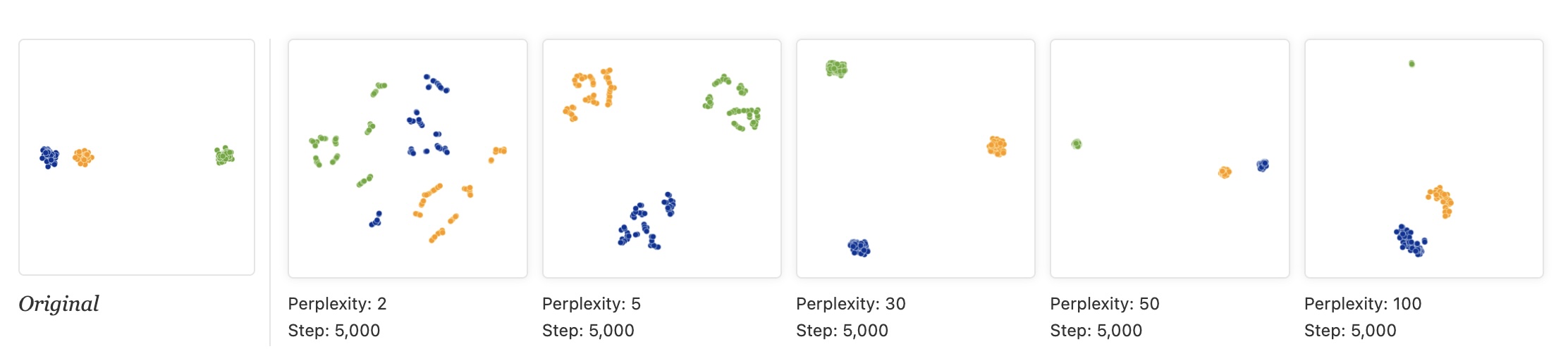
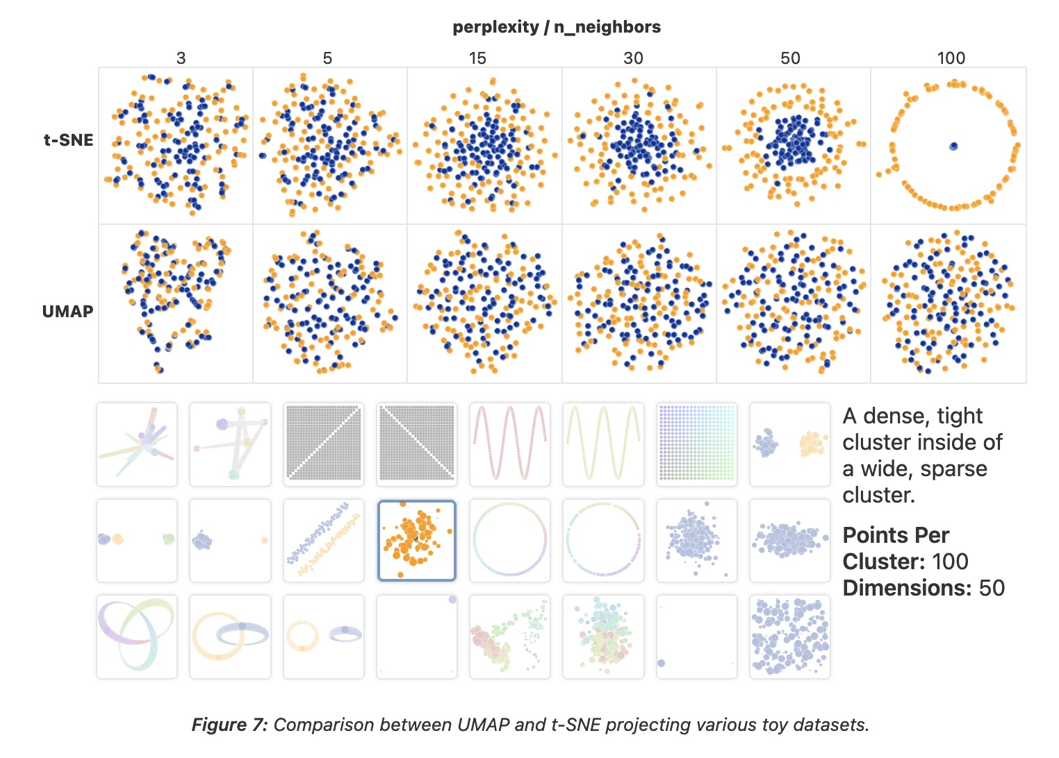
Key Warning: Parameters Matter!

  • t-SNE has a critical parameter: perplexity
    • Roughly the number of close neighbors each point has
    • Typical values: 5-50
    • Different perplexities = different structures!

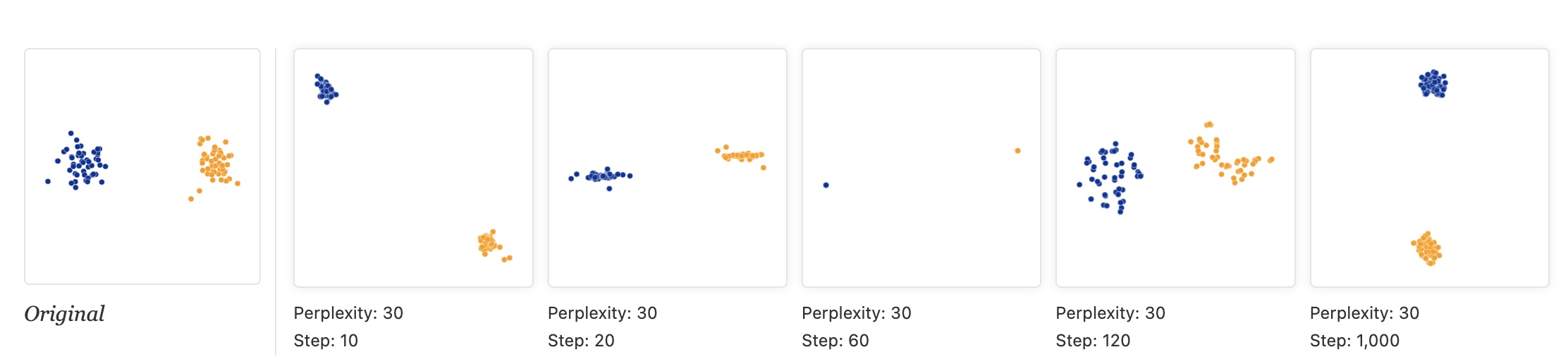
Convergence: Run Enough Iterations!

Critical: Cluster Sizes Mean Nothing!

  • t-SNE equalizes cluster densities
  • Large visual clusters ≠ large actual clusters
  • Size refers to spatial extent, not number of points

Critical: Distances Between Clusters Mean Nothing!

Warning: Random Noise Can Look Structured

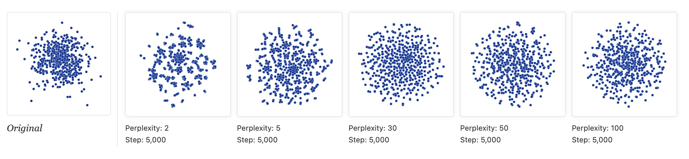
  • Left: PCA of random data (correctly shows no structure)
  • Right: t-SNE of same data (shows apparent clusters!)
  • Lesson: Don’t assume clusters in t-SNE are real!

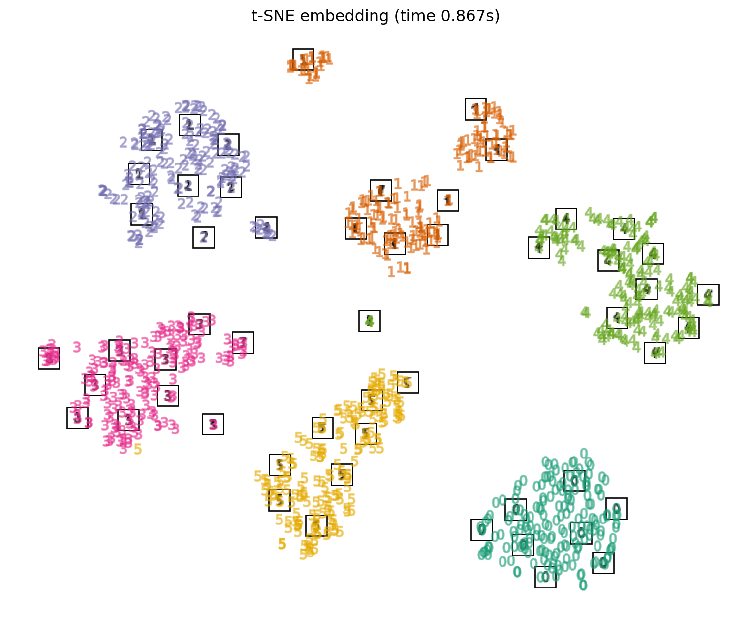
t-SNE Applied to Digits

Non-linear Methods: UMAP

UMAP: The Modern Alternative

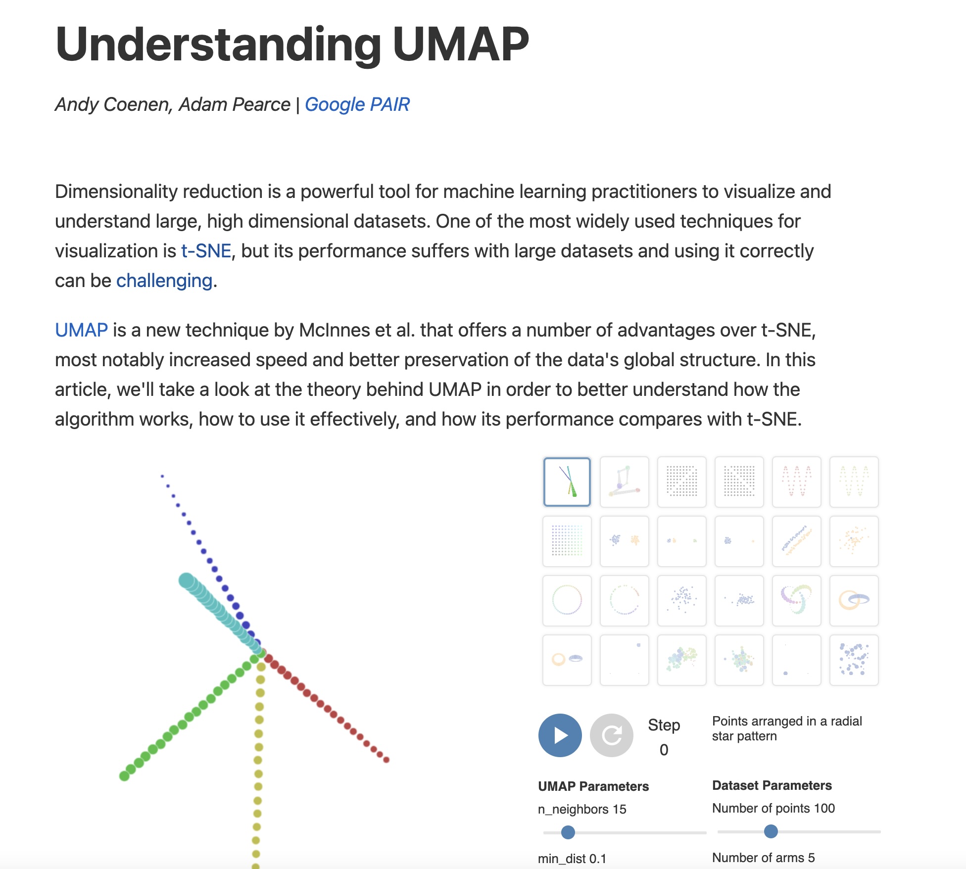
https://pair-code.github.io/understanding-umap/

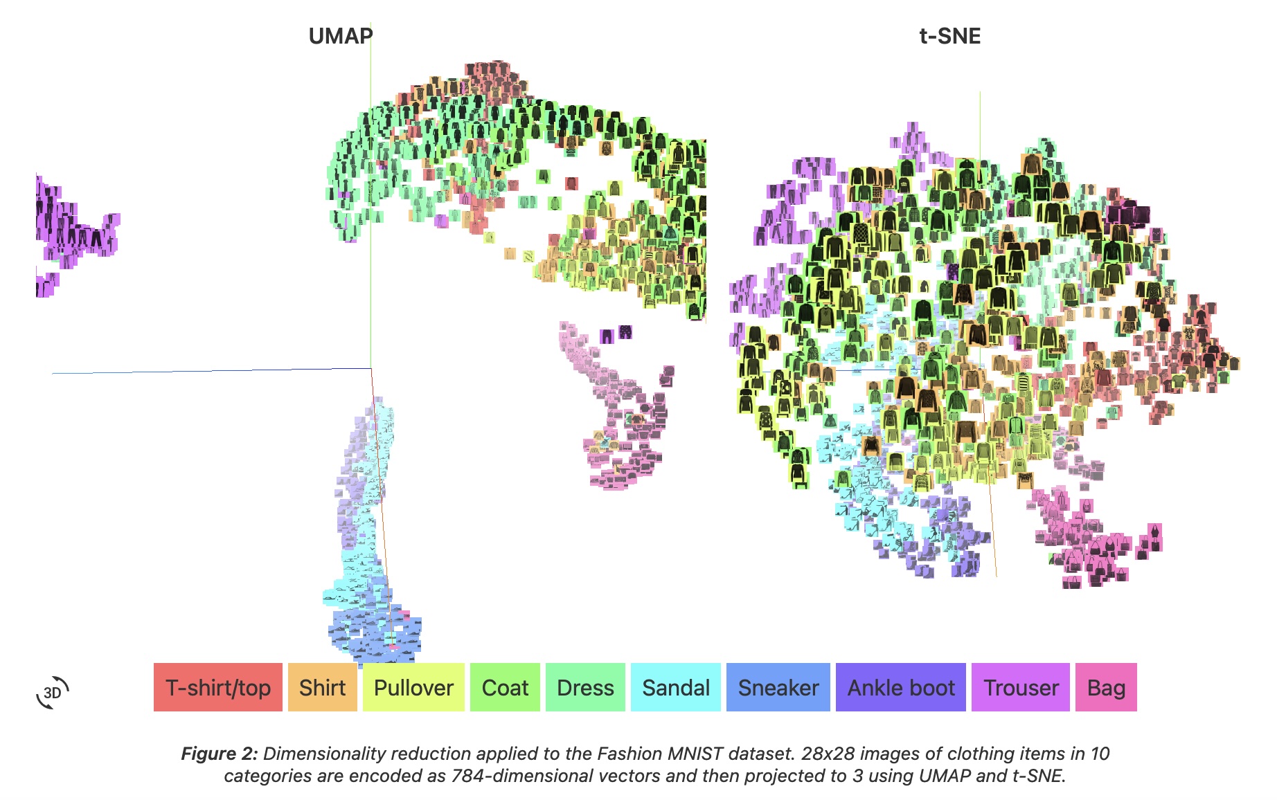
UMAP vs t-SNE: Speed and Structure

  • Speed: UMAP is 10-15x faster than t-SNE
    • MNIST (70K points, 784D): UMAP = 3 min, t-SNE = 45 min!
  • Global structure: UMAP better preserves relationships between clusters
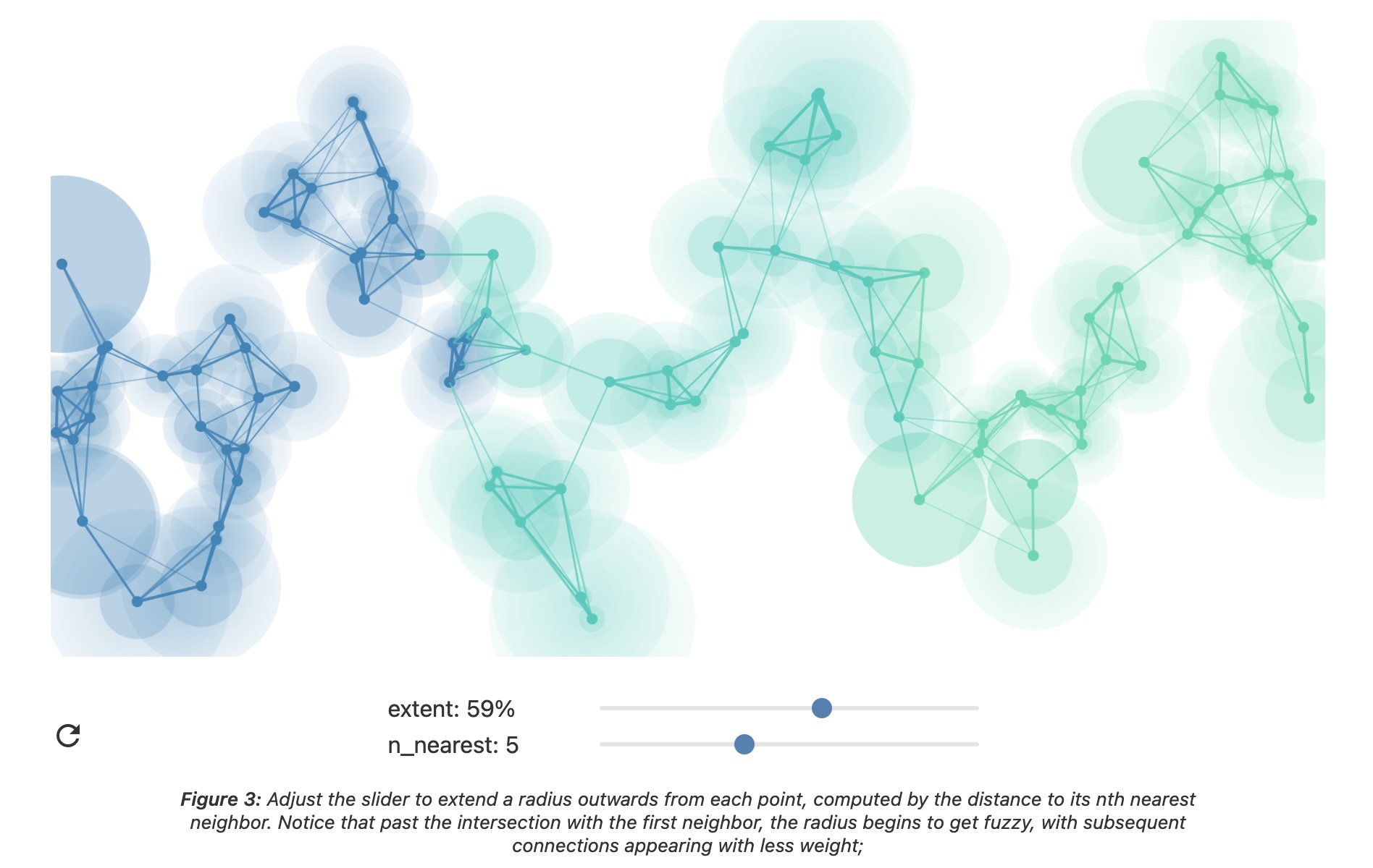
How UMAP Works

UMAP Parameters

  • n_neighbors - balances local vs global structure
    • Low (2-5): very local structure
    • High (50-200): more global structure
    • Similar to t-SNE’s perplexity
  • min_dist - minimum spacing between points
    • Low (0.0): tight clusters
    • High (0.5-0.8): spread out points

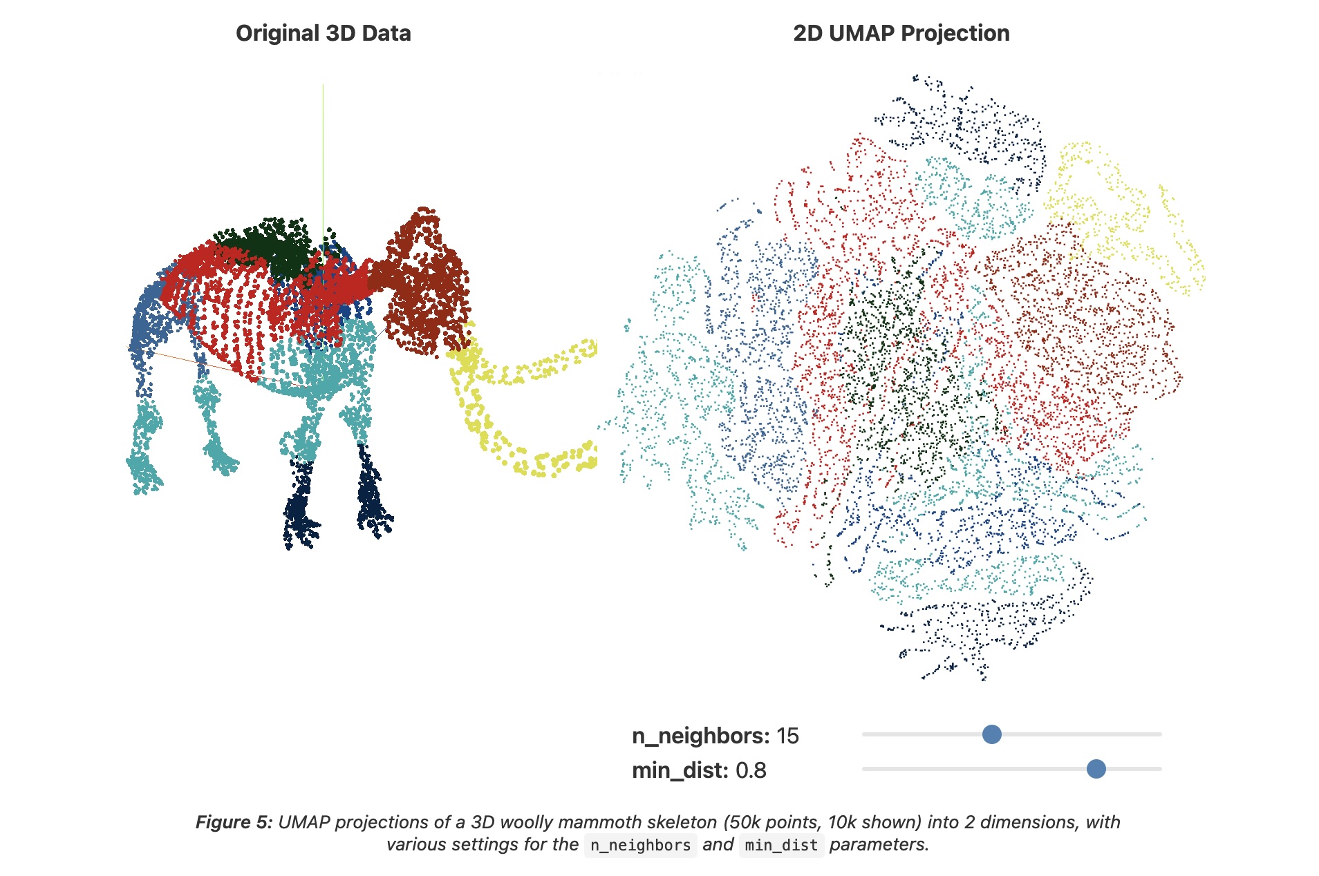
UMAP: min_dist = 0.0

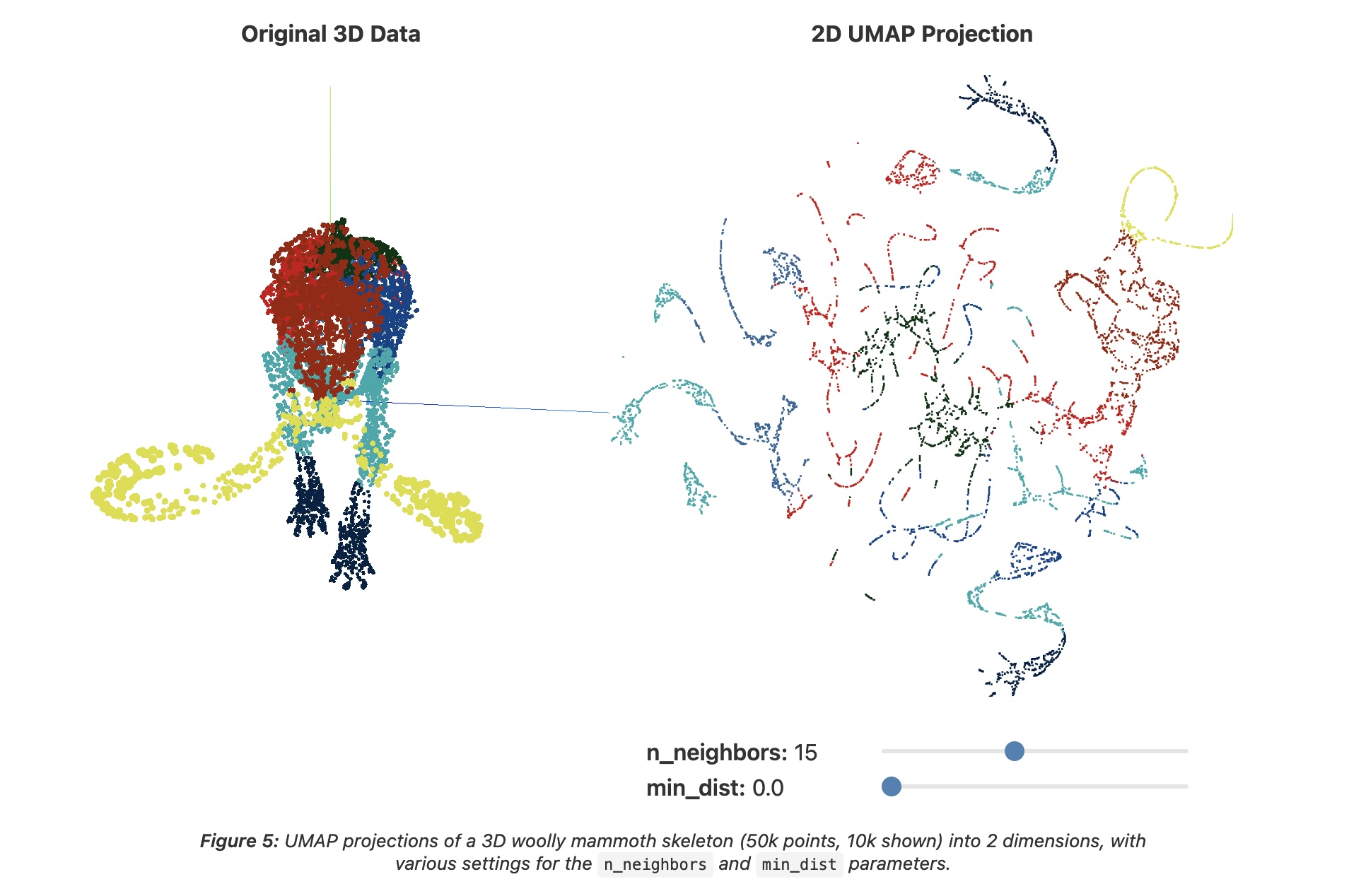
UMAP: min_dist = 0.8

UMAP: Critical Warnings Still Apply!

  • UMAP is non-linear like t-SNE
  • Distances are not directly interpretable
  • Global positioning is better than t-SNE but still not perfect
  • Always try multiple parameter values
  • Validate findings with domain knowledge

Parameter Comparison: t-SNE vs UMAP

Visualization Best Practices

Dimensionality Reduction: Visualization Guidelines

  1. Always show multiple views
    • PCA (linear baseline)
    • t-SNE or UMAP (non-linear)
    • Try multiple parameters
  2. Don’t over-interpret
    • Cluster sizes may be misleading
    • Inter-cluster distances may be unreliable
    • Some structure may be artifacts
  3. Validate findings
    • Check against domain knowledge
    • Use complementary analyses
    • Be transparent about limitations

Interactive Dimensionality Reduction

Summary

  • Clustering helps discover natural groups in data
    • Multiple methods reveal different structures
    • Visualization is essential for interpretation
  • Dimensionality Reduction enables visualization of complex data
    • PCA: fast, interpretable, linear
    • t-SNE: excellent clusters, requires care
    • UMAP: faster, better global structure
  • Critical: Always validate, try multiple methods, understand limitations

Resources and Further Reading

Clustering: * Wolfram Clustering Tutorial * Cluster Analysis (Wikipedia)

Dimensionality Reduction: * How to Use t-SNE Effectively (Essential!) * Understanding UMAP * Dimensionality Reduction (Wikipedia)