Visualizing Network Data

CS-GY 6313 - Fall 2025

Claudio Silva

2025-11-26

Introduction

Based on materials by Enrico Bertini NYU Tandon School of Engineering

LECTURE TIMING GUIDANCE (150 min total)

Part 1: Networks (70 min) - Network fundamentals (10 min) - Force-directed layouts (20 min) - Fixed layouts & edge bundling (15 min) - Matrices & clutter reduction (15 min) - Wrap-up & quiz (10 min)

Part 2: Trees (70 min) - Tree fundamentals (10 min) - Node-link trees & examples (15 min) - Dendrograms (10 min) - Decision trees (10 min) - Treemaps (20 min) - Sunburst/Icicle plots (5 min)

Wrap-up (10 min) - Summary & programming assignments

Part 1: Networks

Objects, relationships, and visualization approaches

Network Data Fundamentals

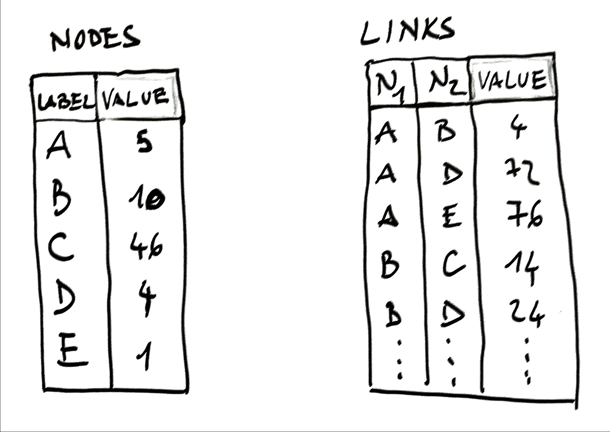
Network Data = Objects + Relationships + Values

• Objects: Nodes (people, cities, genes)
• Relationships: Edges (friendships, routes, interactions)
• Values: Node attributes (age, size) & edge attributes (weight, type)

Application Domains: Social networks, biological systems, transportation, web, infrastructure

• Network data is one of the most fundamental data structures
• Key distinction: We care about RELATIONSHIPS, not just entities
• Ask: “What networks do you interact with daily?”
• Examples: Facebook (social), protein networks (biological), airline routes (transportation)
• Values/attributes make networks meaningful beyond pure structure

Example: Friendship Network

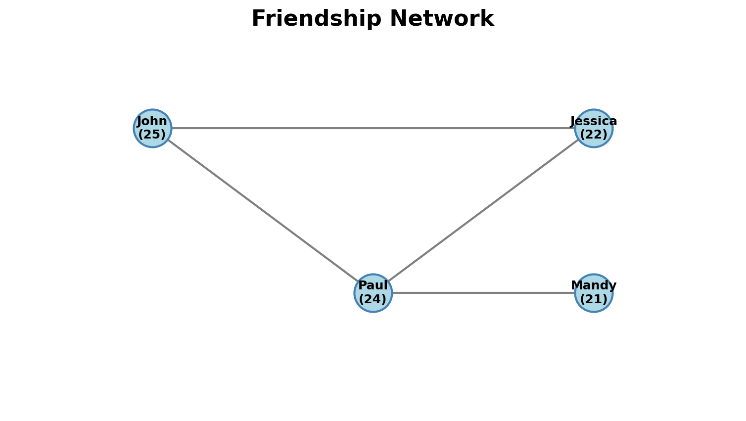
• Nodes: People with attributes (name, age)
• Edges: Friendship connections
• Attributes: Could encode strength, duration, message count

• Concrete example to ground abstract concepts
• This is undirected (friendship is mutual)
• Later: directed graphs (Twitter follows, citations)
• Question: “How would you find the most connected person?”

Fundamental Approaches

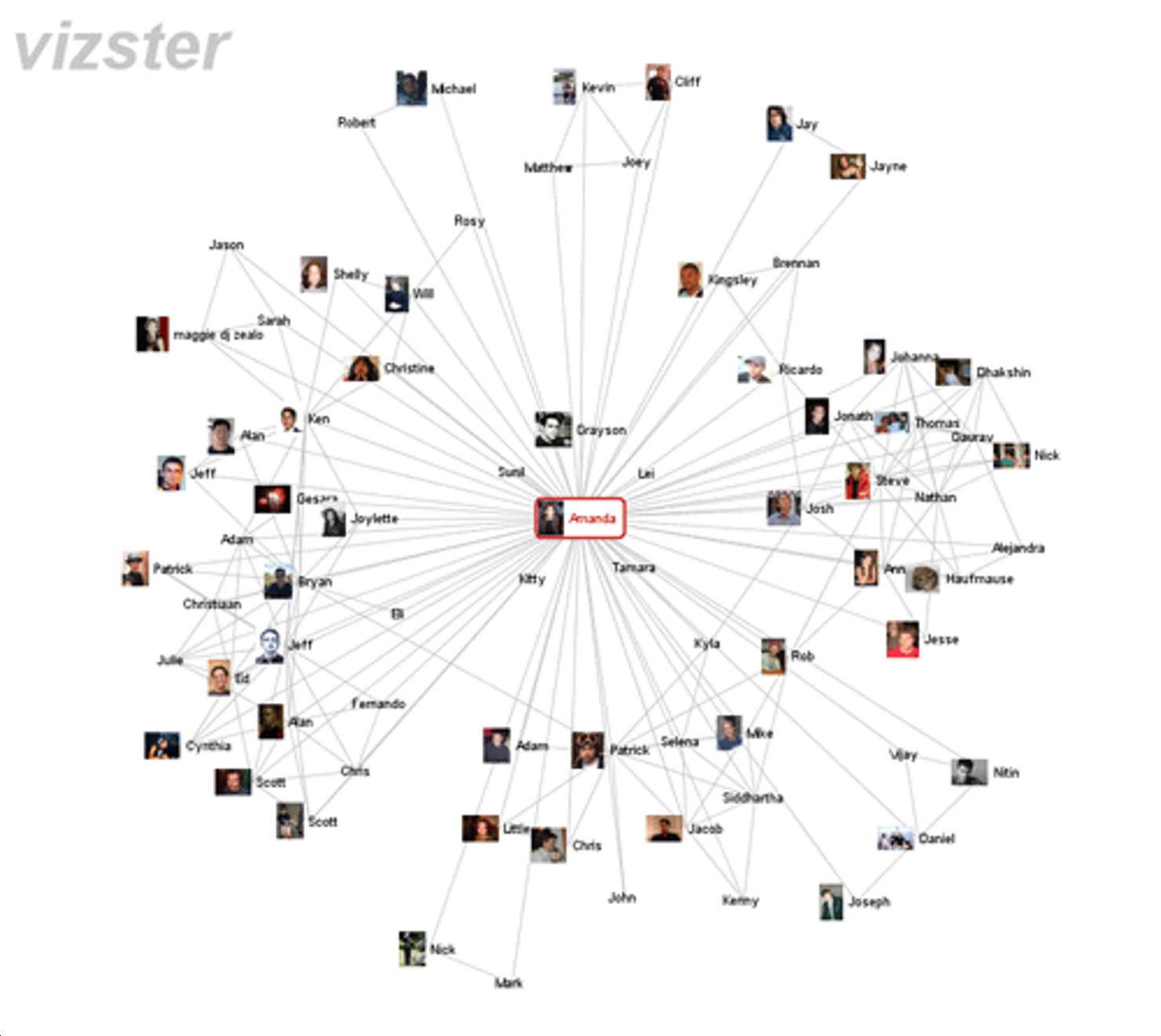
1. Node-Link Diagrams

• Nodes = dots/markers
• Edges = connecting lines
• Two types: Force-directed (algorithmic) & Fixed (meaningful positions)

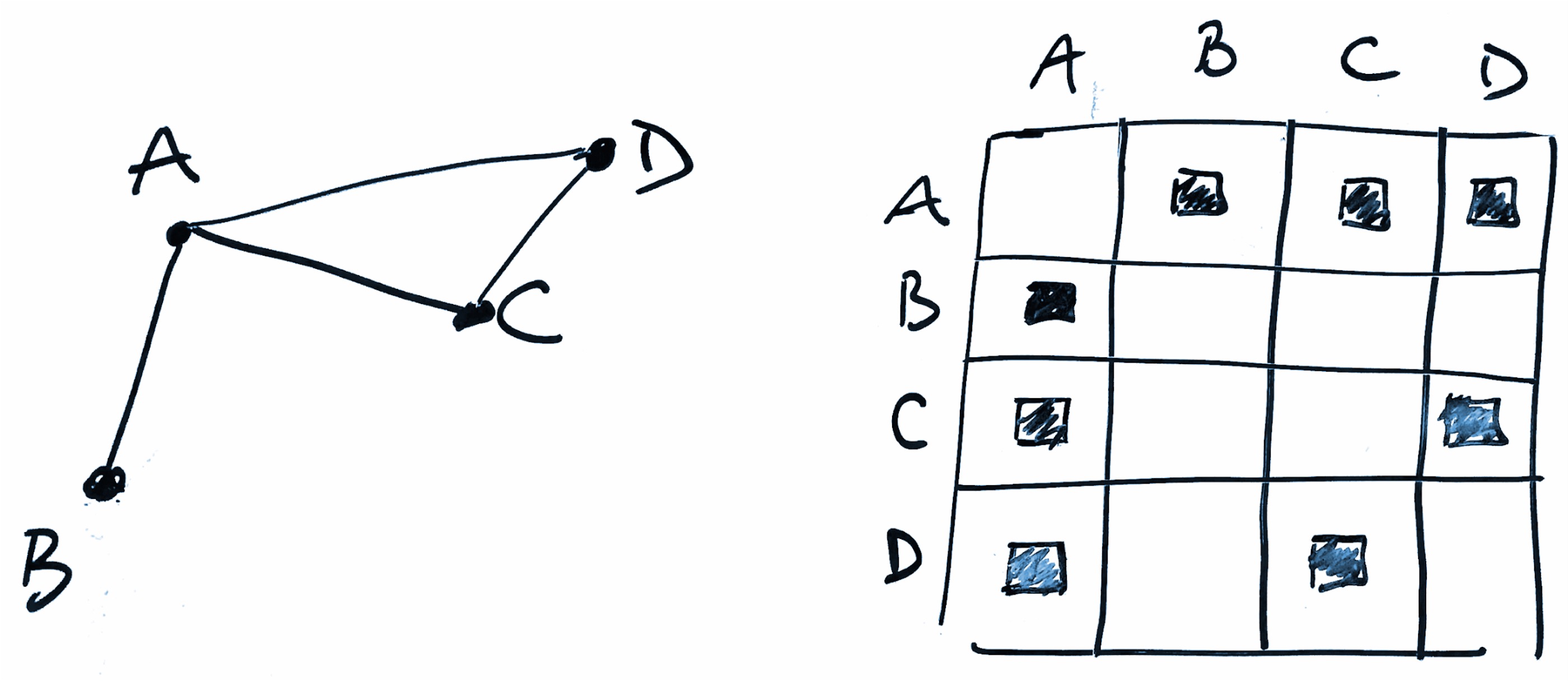
2. Adjacency Matrices

• Rows & columns = nodes
• Cells = edges
• No line crossings, but less intuitive

Force-Directed

Matrix

• Two fundamental paradigms - trade-offs between them
• Node-link: Intuitive, shows structure, but clutters
• Matrix: Scalable, precise, but unfamiliar

Force-Directed Layouts

Physics simulation for automatic positioning

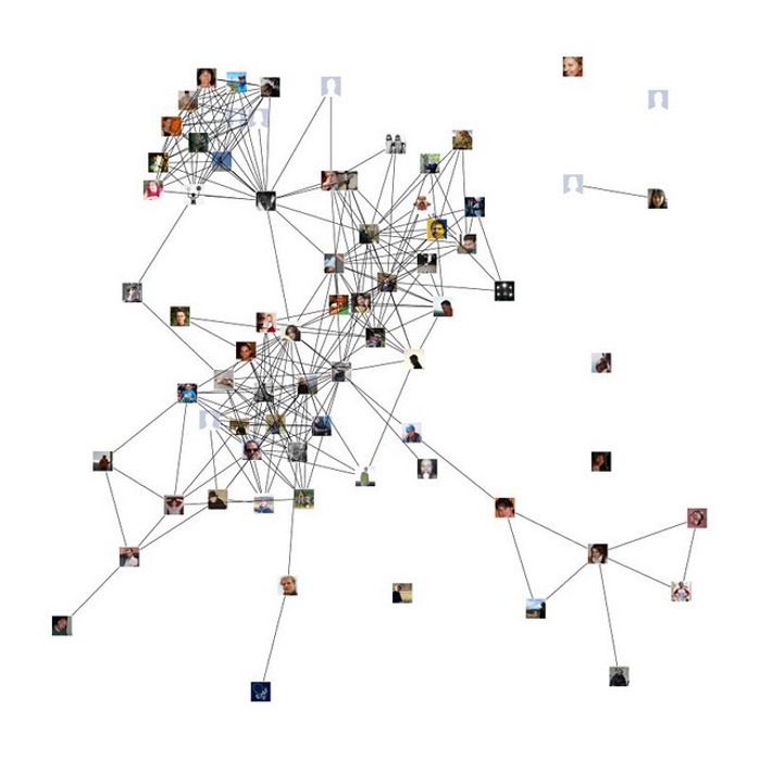
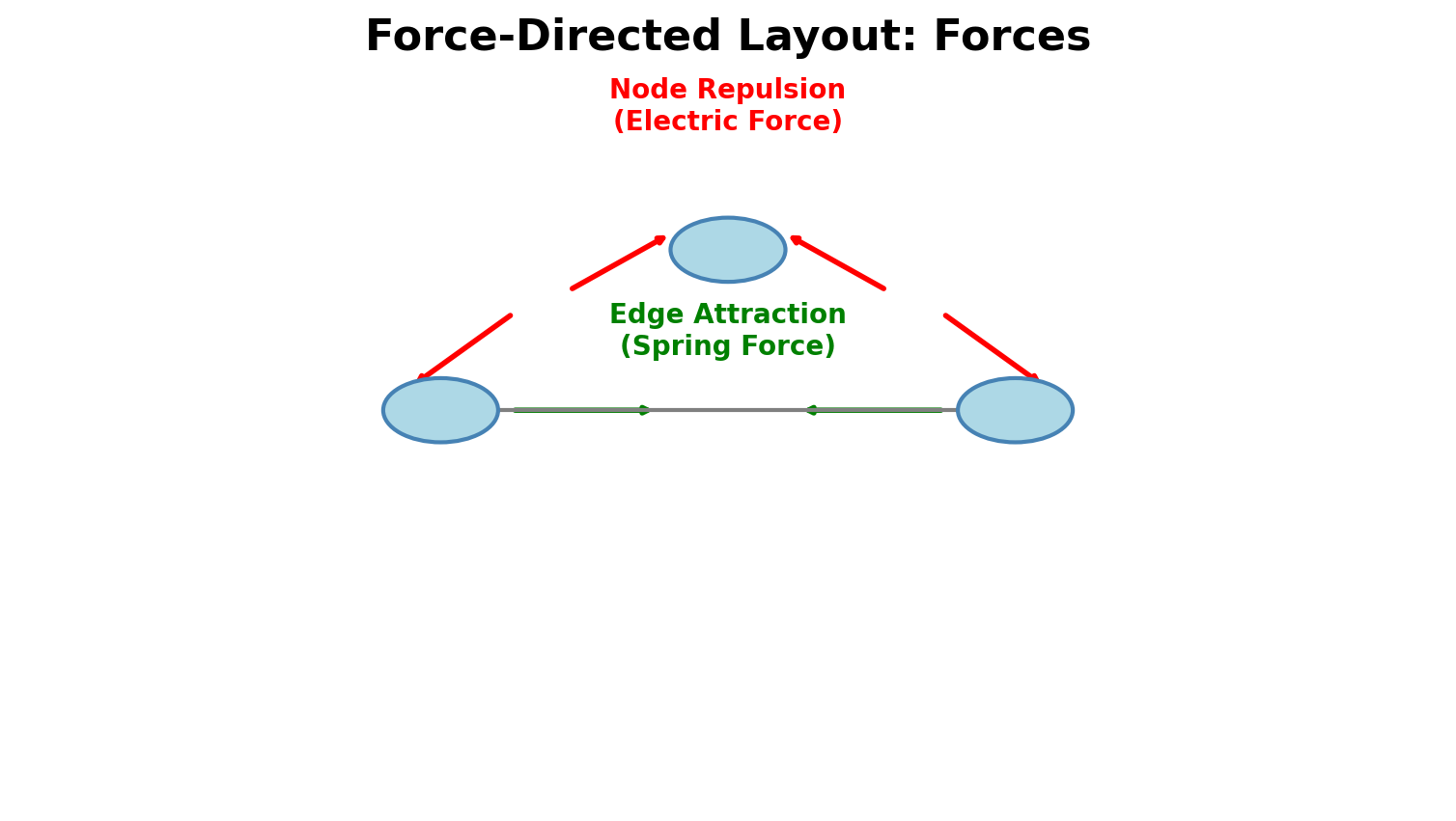
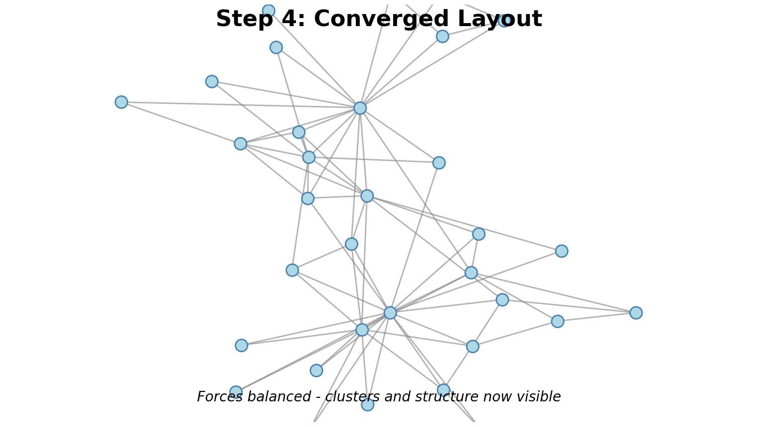
Force-Directed: How It Works

Physical Analogy:

• Edge Attraction: Connected nodes pull together (springs)
• Node Repulsion: All nodes push apart (charged particles)
• System evolves until forces balance

Result: Clusters emerge, bridges visible, hubs toward center

• Treat network as physical system - let physics arrange it
• NOT “correct” layout (networks have no inherent positions)
• BUT: Often reveals meaningful structure
• Many variants: Fruchterman-Reingold, Kamada-Kawai, ForceAtlas2, D3 force

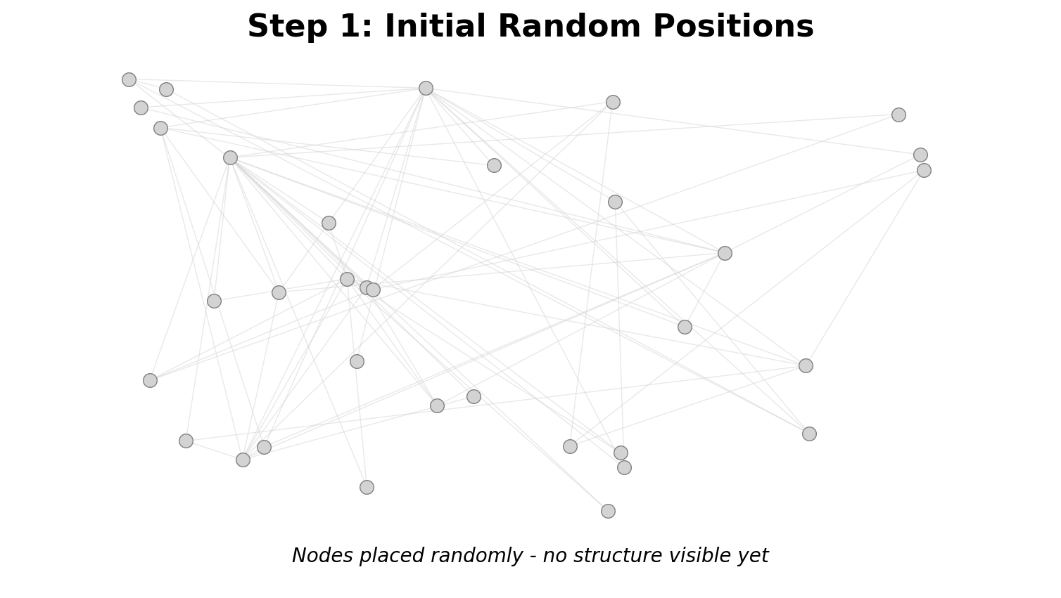
Force-Directed Algorithm

Steps:

1. Initialize: Random positions
2. Calculate: Net force on each node (attraction + repulsion)
3. Move: Displace nodes by force × step_size
4. Iterate: Repeat until convergence (50-500 iterations)

Complexity: O(n²) per iteration (expensive for large networks)

Step 1: Random

Step 4: Converged

• Start: Chaos (random dots)
• End: Structure (organized, balanced)
• Convergence criteria: low energy, max iterations, or negligible changes
• Modern optimizations use Barnes-Hut for O(n log n)

Visual Encoding on Nodes & Edges

Node Encodings:

• Size: Degree, importance, value
• Color: Category, cluster, metric
• Shape: Type (circles, squares, triangles)

Edge Encodings:

• Thickness: Weight, strength, traffic
• Pattern: Type (solid, dashed, dotted)
• Color: Category, direction

Encoded network

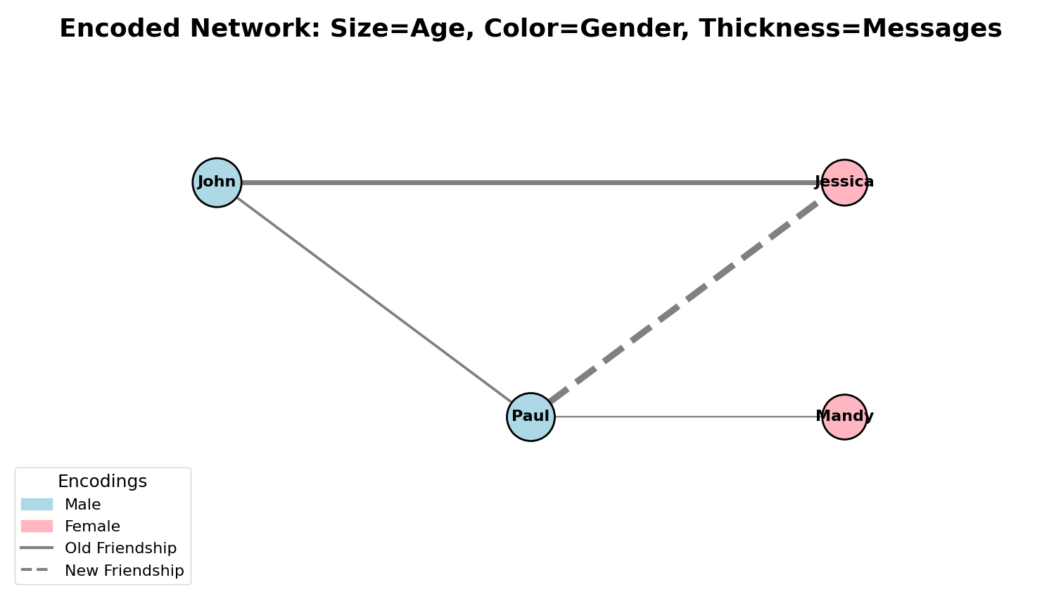
Example: Size=age, Color=gender, Thickness=messages, Pattern=old/new friendship

• Force-directed gives positions, but we have more visual channels!
• Link back to perception lectures: Visual channel hierarchy
• Warning: Don’t over-encode (too complex = unreadable)
• Example shows 4 encodings - approaching the limit

Fixed Layouts

Meaningful node positions instead of algorithmic

Fixed Layouts: When & Why

When to use fixed instead of force-directed:

1. Nodes have meaningful attributes for positioning (geography, time, hierarchy)
2. Emphasizing edges/flows more than clustering
3. Need stable, reproducible layouts

Common patterns: Circular, linear, grid, spatial (geographic)

• Fixed = WE decide positions (not algorithm)
• Trade structure visibility for semantic positioning
• Example: Geographic networks (airports at real locations)

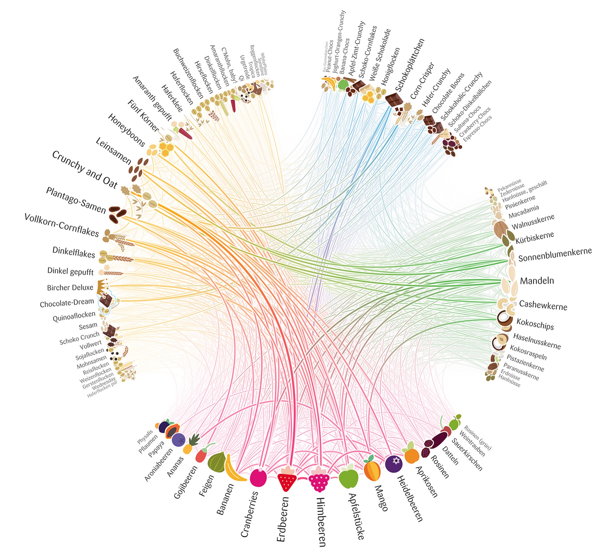
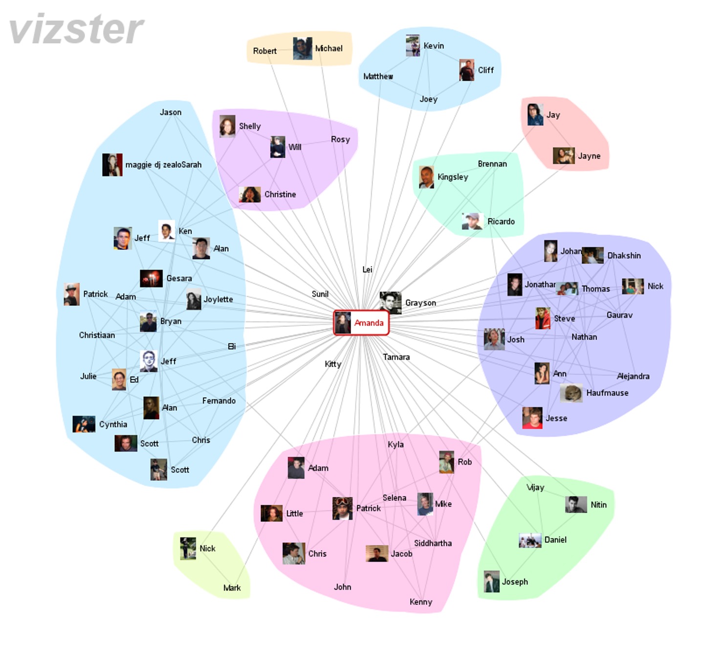
Circular Layouts & Edge Bundling

Circular Layout:

• Nodes evenly distributed around circle
• Critical decision: Node ordering (alphabetical? by cluster? to minimize crossings?)

Edge Bundling:

• Route similar edges along common paths
• Reduces clutter, reveals flow patterns

Hierarchical Edge Bundling

• Node order matters! Different orders reveal different patterns
• Edge bundling: Trade individual edge traceability for overall flow visibility
• Holten’s 2006 paper hugely influential - thousands of citations

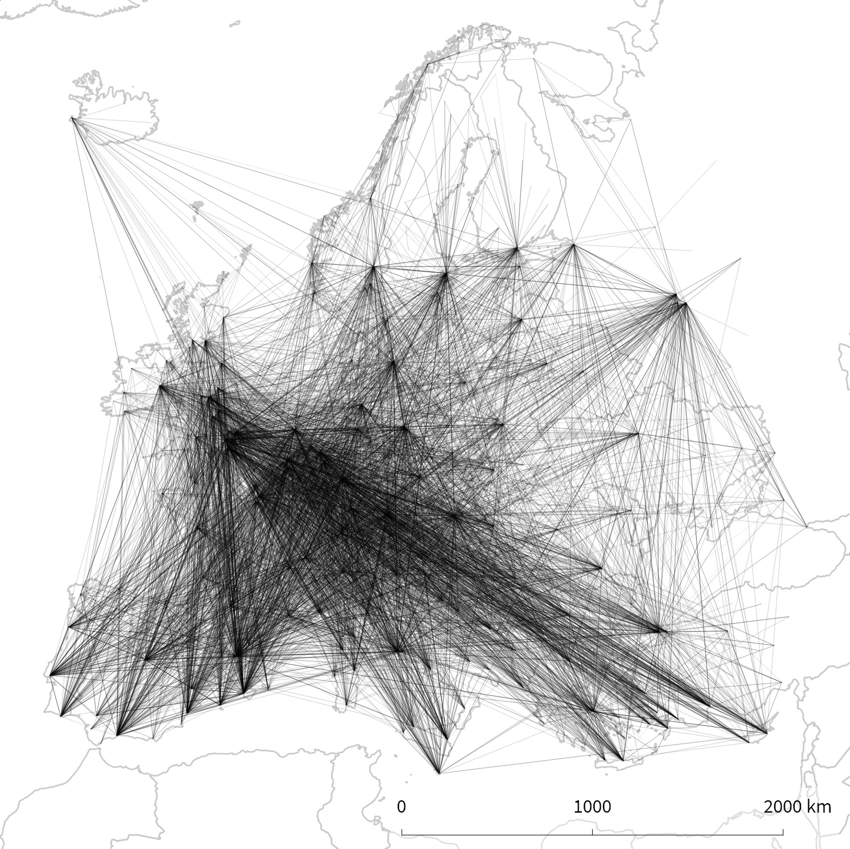
Spatial Networks & Bundling

Geographic Networks: Nodes at real locations (airports, cities, servers)

Problem: Edge clutter!

Solution: Edge bundling reveals corridors, hubs, regional patterns

Tools: qGIS, Gephi, D3.js

Before: Cluttered

After: Bundled

• Classic example: European flight network
• Before: Spaghetti! Can’t see anything
• After: Major travel corridors, hub cities visible
• Use when aggregate patterns > individual connections

Adjacency Matrices

Table representation of networks

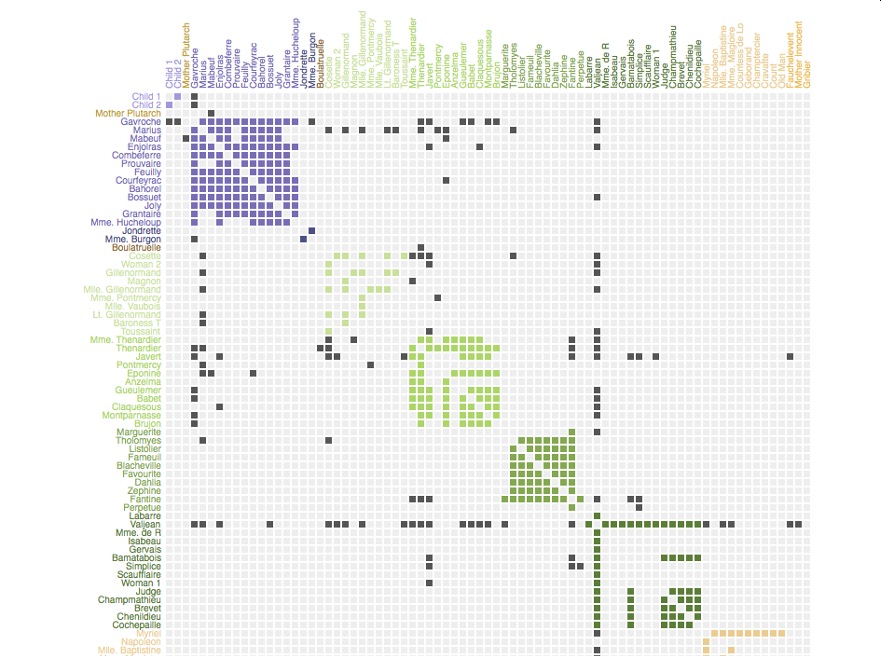
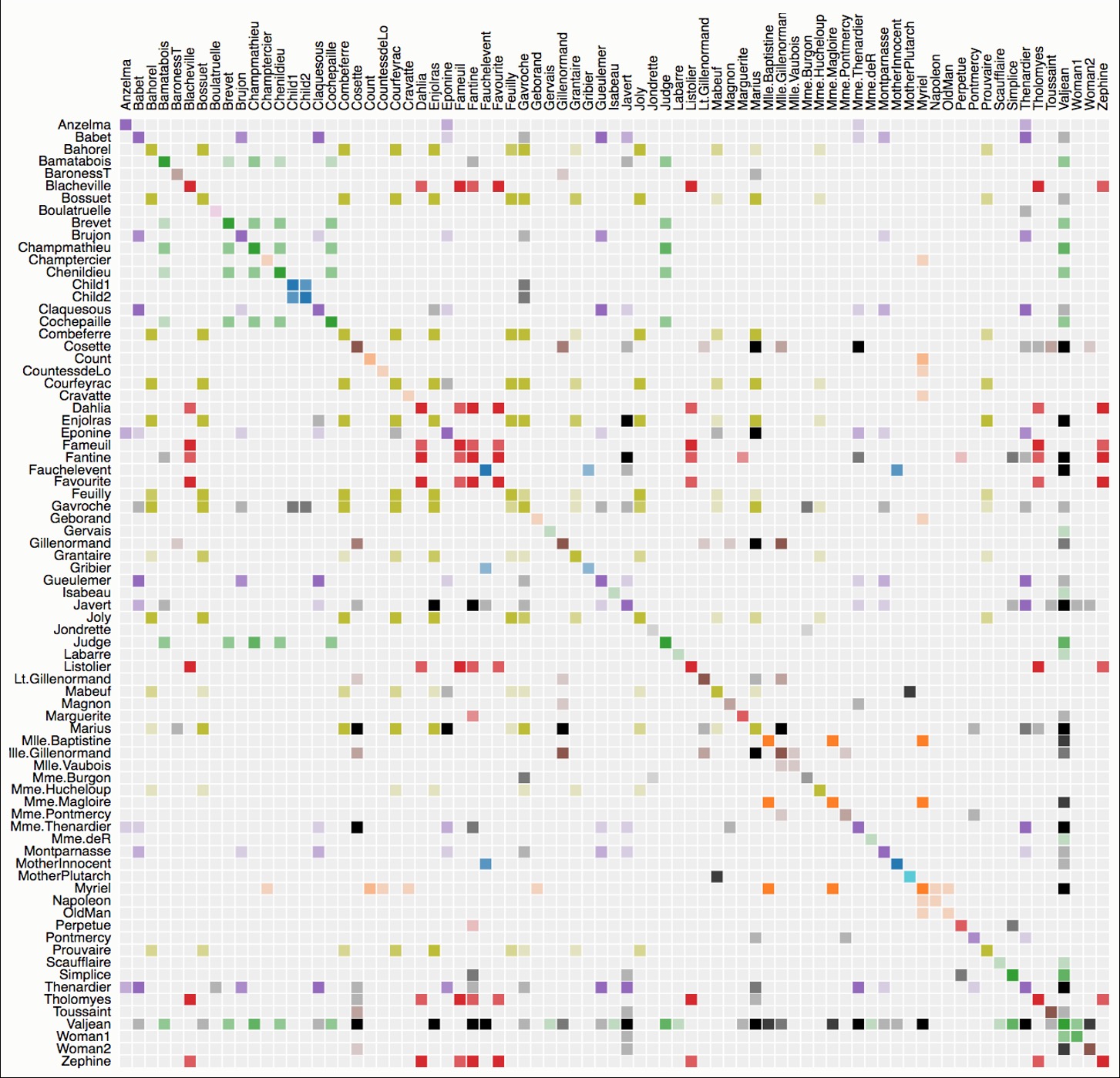
Matrices: Concept & Trade-offs

Encoding:

• Rows & columns = nodes
• Cell (i,j) = edge from node i to j
• Color/symbol = edge weight/presence

Advantages: ✓ All nodes visible, ✓ No crossings, ✓ Scalable to denser networks

Disadvantages: ✗ Less intuitive, ✗ Needs reordering, ✗ n² space, ✗ Hard to trace paths

Network → Matrix

Les Misérables

• Completely different paradigm from node-link
• User studies: Experts faster with matrices, novices prefer node-link
• Task matters: Degree queries easier with matrices, path queries easier with node-link

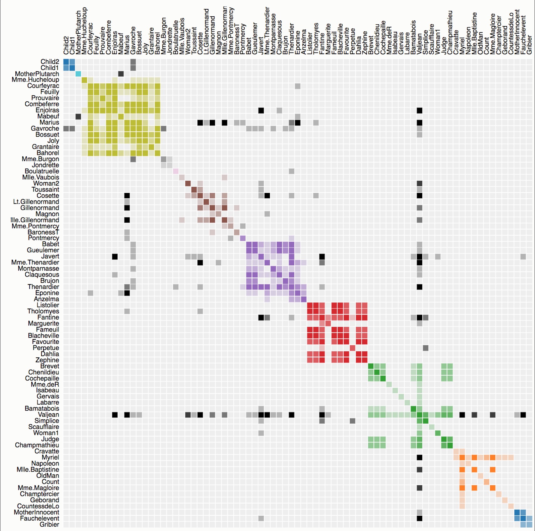
The Hairball Problem & Matrix Ordering

“Hairball”: Dense networks as node-link diagrams = unreadable

Solution: Switch to matrix OR apply clutter reduction

Critical: Matrix ordering reveals patterns!

Hairball

• Hairball = technical term for unreadable dense node-link
• Ordering is critical design parameter (like aspect ratio for line charts)
• Strategies: alphabetical, by degree, clustering, seriation algorithms
• NP-hard to find optimal ordering

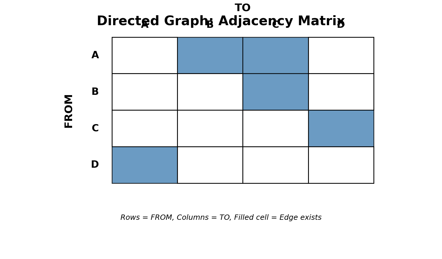
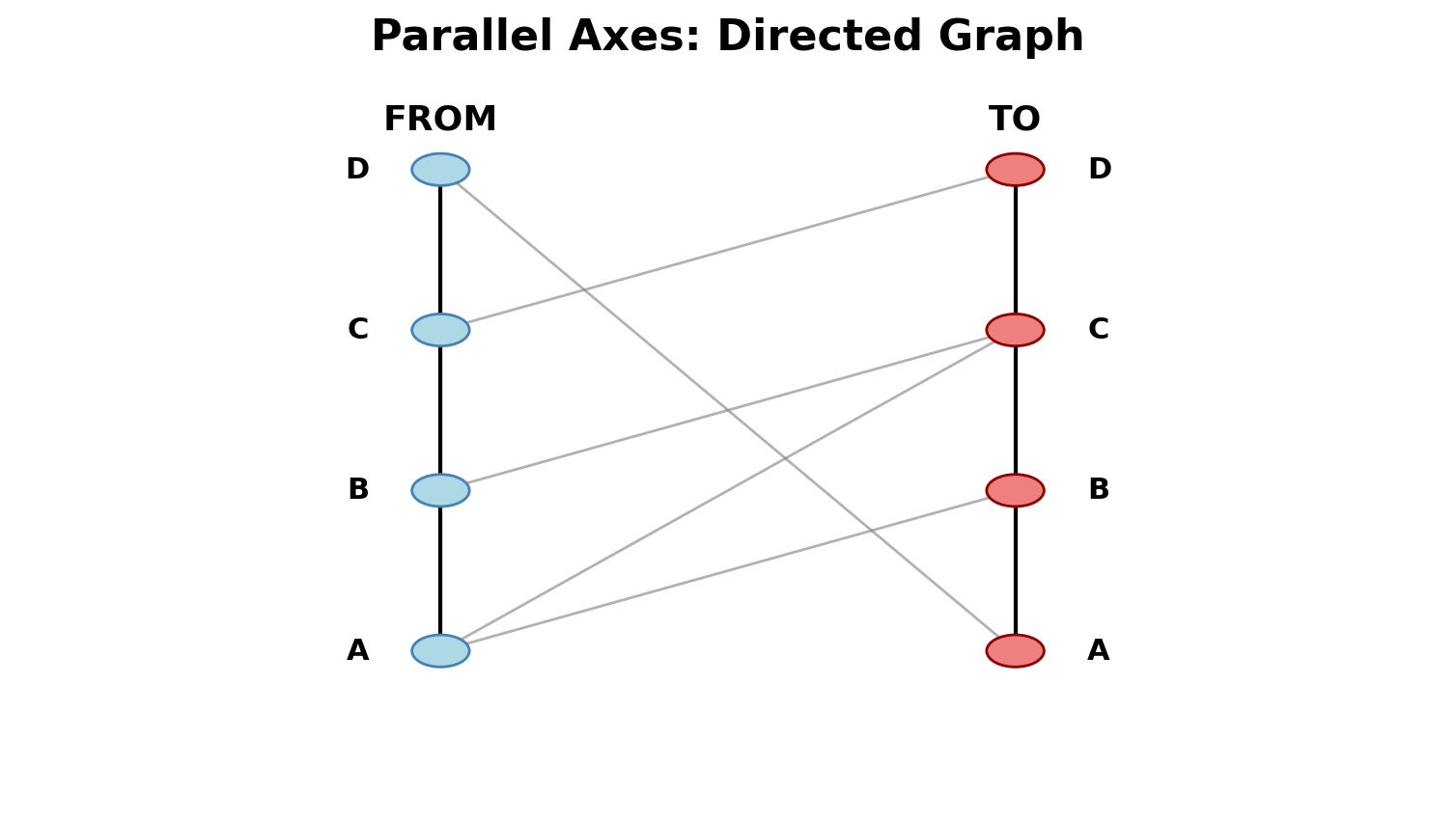
Directed Graphs & Alternatives

Directed Matrices:

• Asymmetric: (i,j) ≠ (j,i)
• Above diagonal = one direction
• Below diagonal = opposite direction
• Easy to see reciprocity

Alternative: Parallel axes (bipartite-like view)

Directed Matrix

Parallel Axes

• Directed graphs: Twitter follows, citations, email, transactions
• Matrix naturally handles direction (no overlapping arrows)
• Parallel axes: Compact, shows in/out degree, but edges cross

Clutter Reduction Strategies

Five main techniques:

1. Edge Bundling: Route similar edges together
2. Clustering: Group nodes into super-nodes
3. Filtering: Show subset (threshold, top-k, backbone)
4. On-Demand: Show edges only on hover/click
5. Motif Simplification: Replace patterns with glyphs (cliques, stars → symbols)

• Dense networks need strategies to make them comprehensible
• Often combine multiple techniques (bundle + cluster + filter)
• Trade detail for clarity
• Best practice: Progressive disclosure (overview → drill-down)

Quiz: Fixed vs Force-Directed

Question: The main advantage of a fixed layout over force-directed is:

A. Less cluttered visualizations B. Node positions encode meaningful data C. Faster computation

Answer: B - Position can carry information (geography, time, category)

• A is wrong: Fixed can be MORE cluttered (many crossings)
• C is true but not the MAIN advantage (speed is secondary)
• B is correct: The key benefit is semantic positioning
• Choose fixed when attributes > structure

Part 2: Trees (Hierarchies)

Specialized networks with no cycles

Trees: Definition & Applications

Tree: Network with hierarchical structure, no cycles

Properties:

• One root node
• Parent-child relationships
• Leaves: Nodes with no children
• Unique path between any two nodes

Real-world: File systems, org charts, evolutionary trees, taxonomies, syntax trees

• Trees are everywhere! One of most fundamental data structures
• Hierarchy is natural way humans organize information
• Reduces cognitive load (can’t remember 10,000 items, but can remember 7±2 categories with subcategories)
• This motivates specialized visualization techniques

Two Approaches for Trees

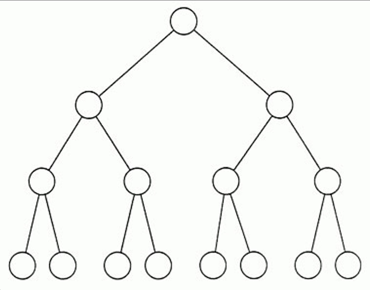
1. Node-Link

• Explicit parent-child connections
• Structure very visible
• Familiar, intuitive
• Limitation: Doesn’t scale (exponential width growth)

2. Space-Filling (Containment)

• Nesting shows hierarchy
• No explicit edges
• Space-efficient, can show size
• Limitation: Structure harder to see

• Fundamental trade-off: Structure vs Scalability
• Node-link: Good for small trees (<100 nodes)
• Space-filling: Good for large trees (1000s of nodes)

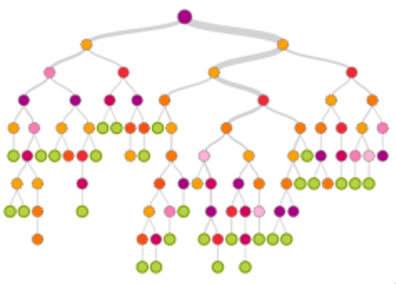
Node-Link Trees: Examples

Top-Down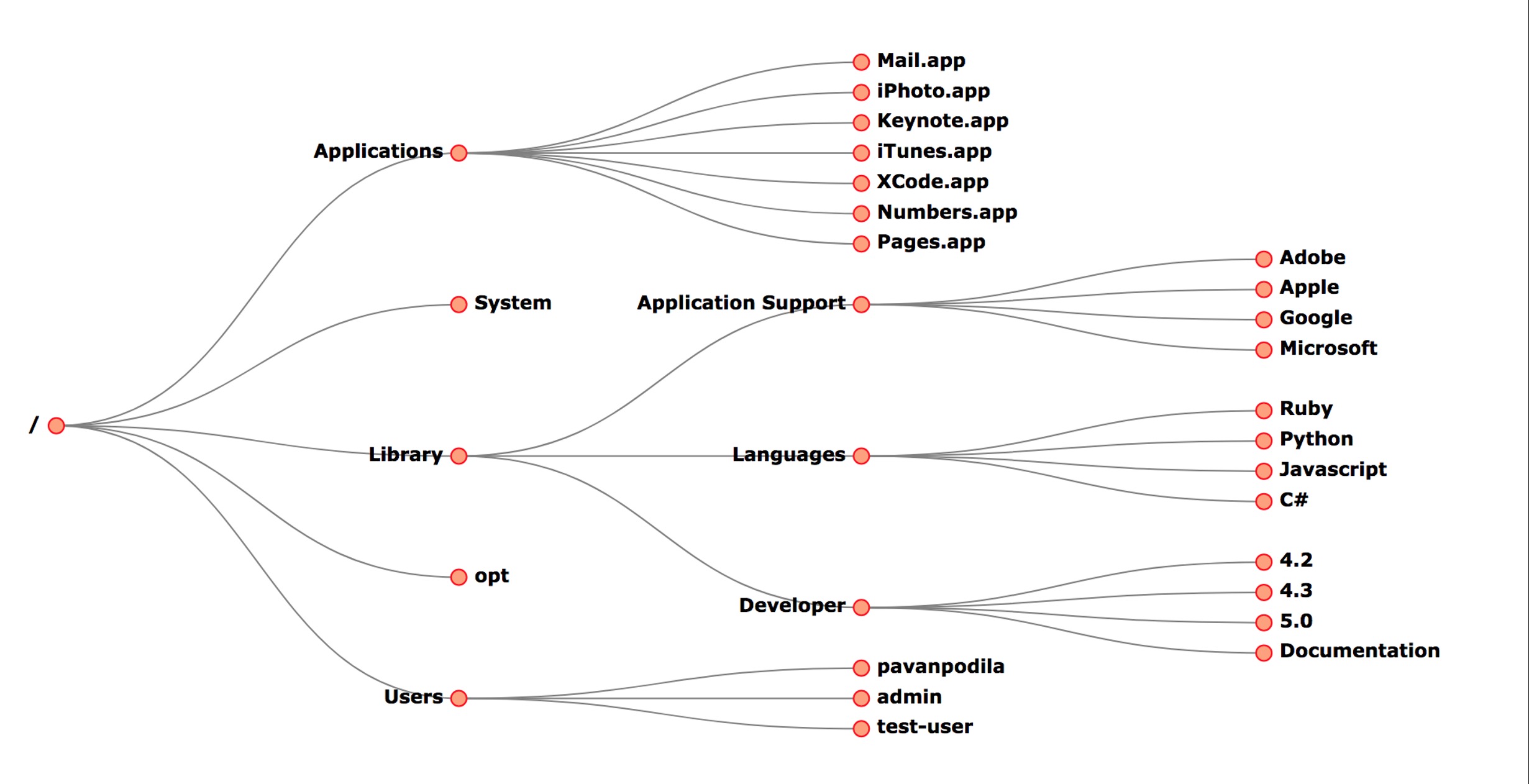

File systems, org charts

Radial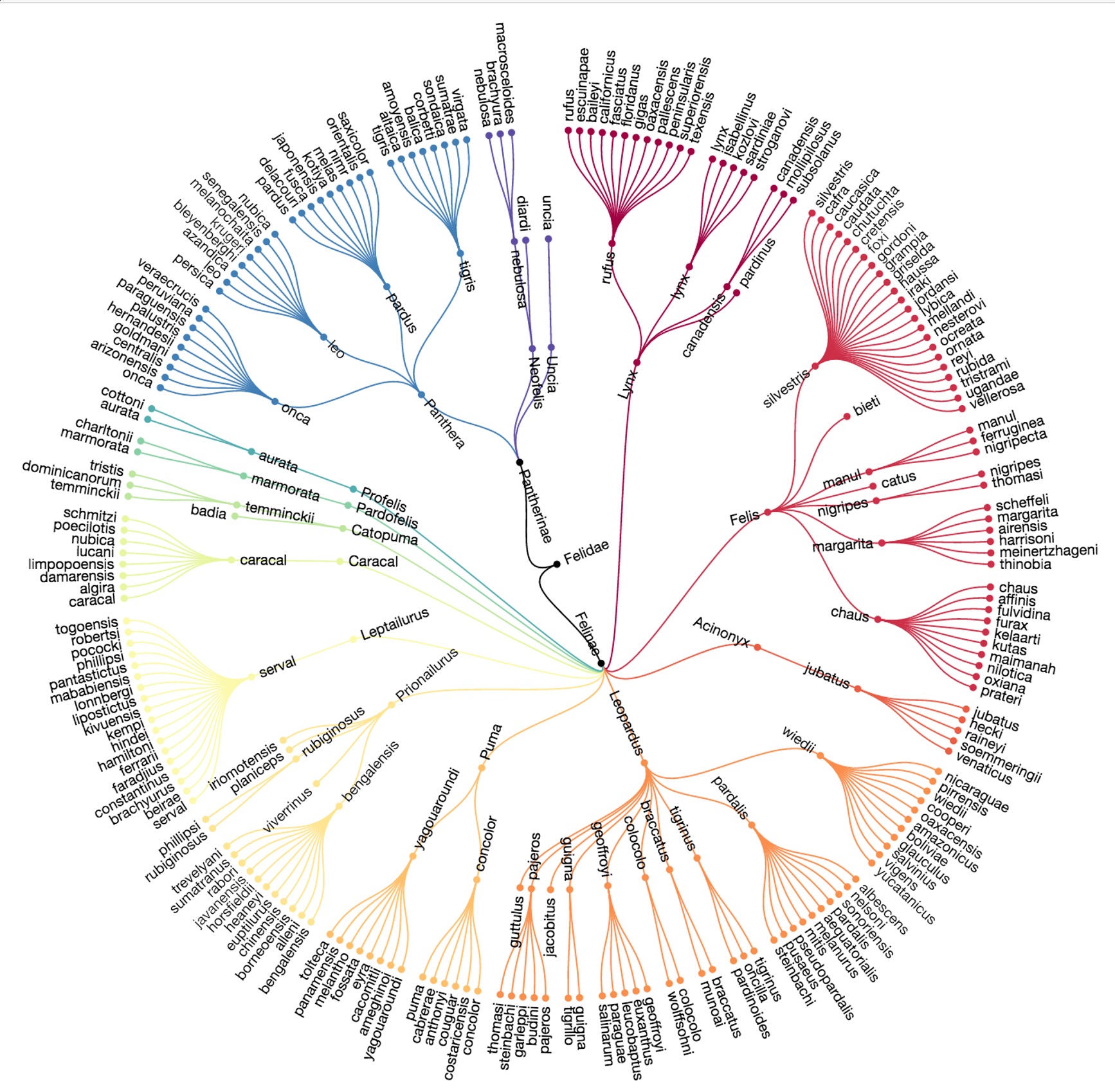

More space-efficient

Indented List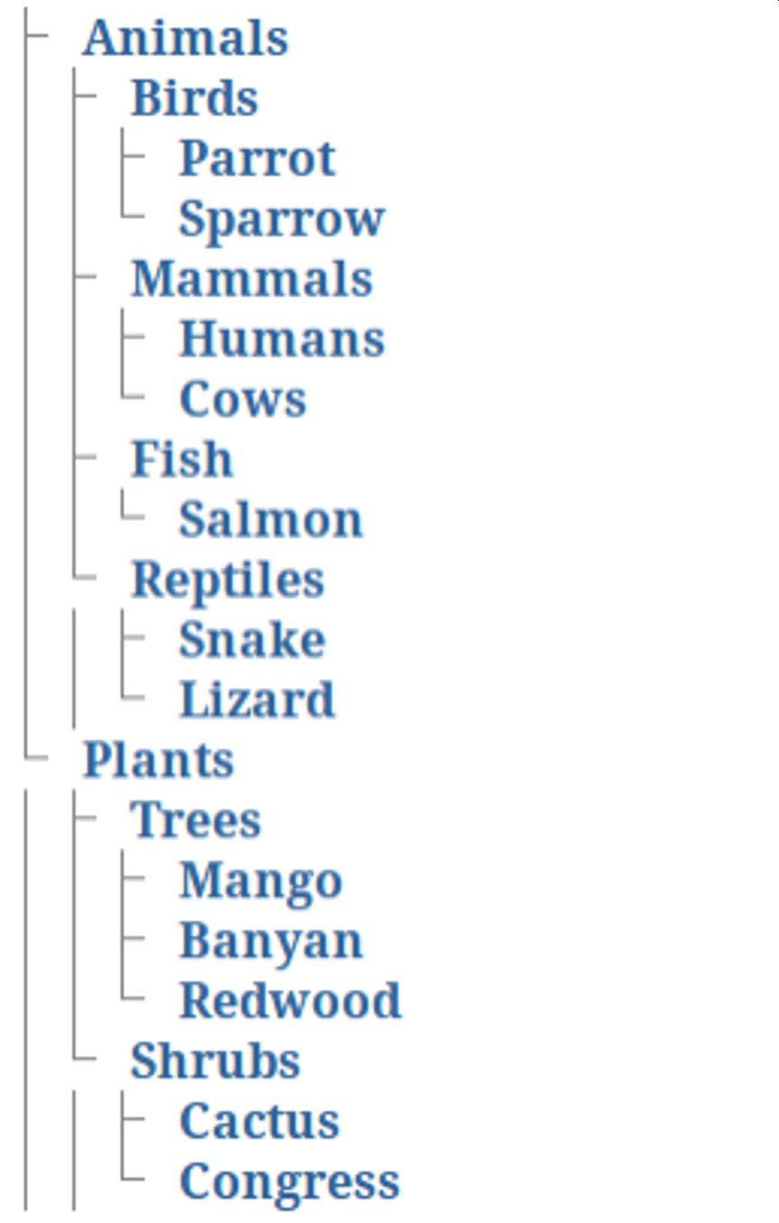

Most compact

Issues: Scalability (1D growth), labeling, limited encoding channels

• Top-down: Most familiar, matches mental model
• Radial: Uses 2D space radially, aesthetically pleasing
• Indented: Most compact, used in file browsers
• All struggle with large/deep trees

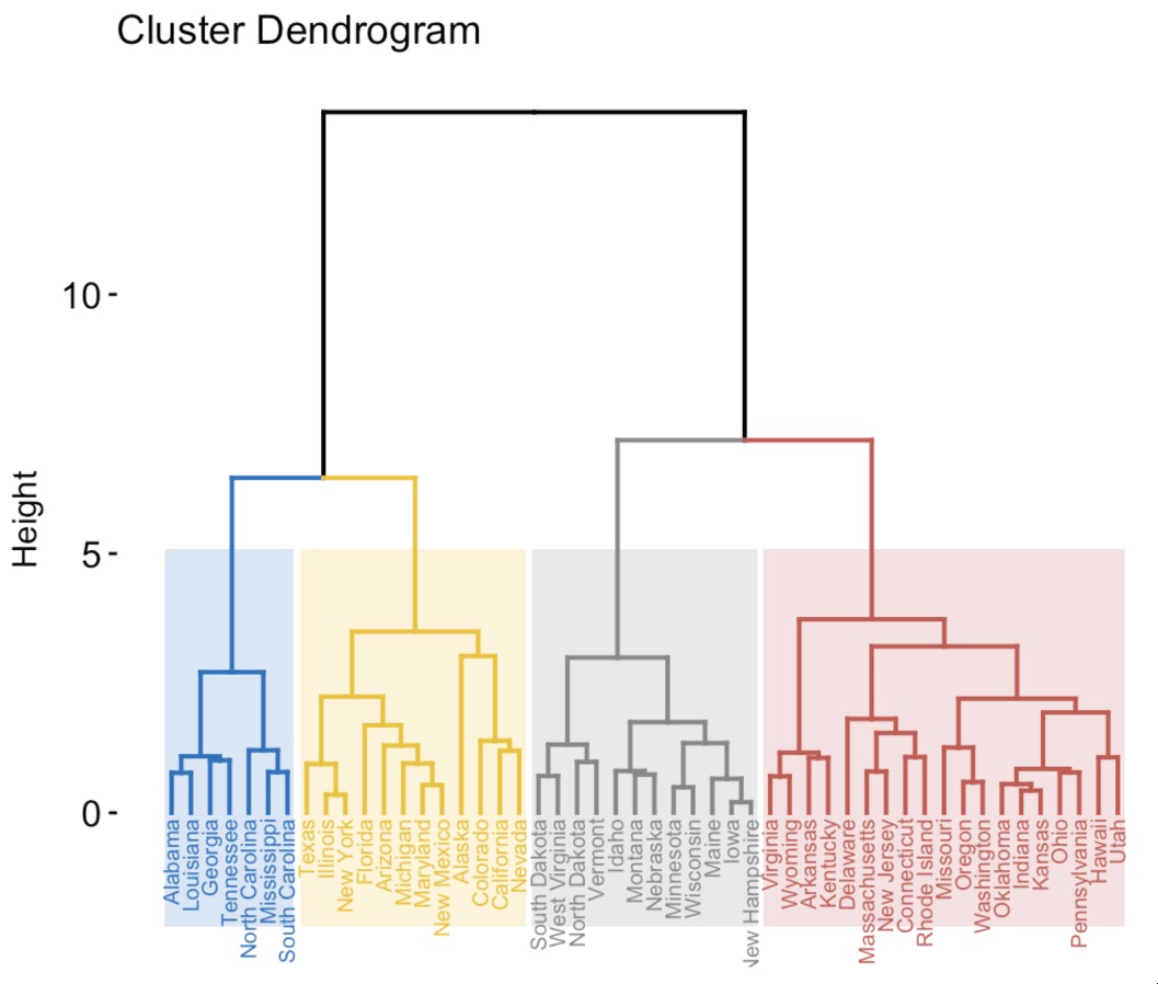
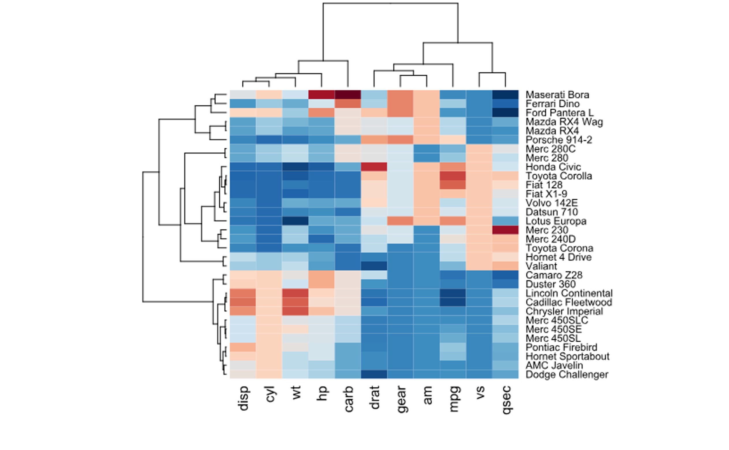
Special Trees: Dendrograms

Dendrogram: Tree showing hierarchical clustering results

Algorithm (Agglomerative): 1. Start: Each point = own cluster 2. Find two closest clusters 3. Merge them (height = distance) 4. Repeat until one cluster

Properties: - Binary tree structure - Branch height = dissimilarity at merge - Cutting at height defines # of clusters

Used in: Gene expression, customer segmentation, document clustering

With Heatmap

• Specific type of tree from hierarchical clustering algorithm
• Branch height is meaningful (unlike layout-only trees where height is just for layout)
• Algorithm is bottom-up: Start with individual points, iteratively merge closest clusters
• Height at which clusters merge represents their dissimilarity
• Cutting dendrogram horizontally at different heights gives different numbers of clusters
• Often paired with heatmaps for multivariate data (shown in image)
• Standard in biology, but useful across any domain where you can define distance/similarity
• Example: Gene expression (cluster genes by similar expression patterns)

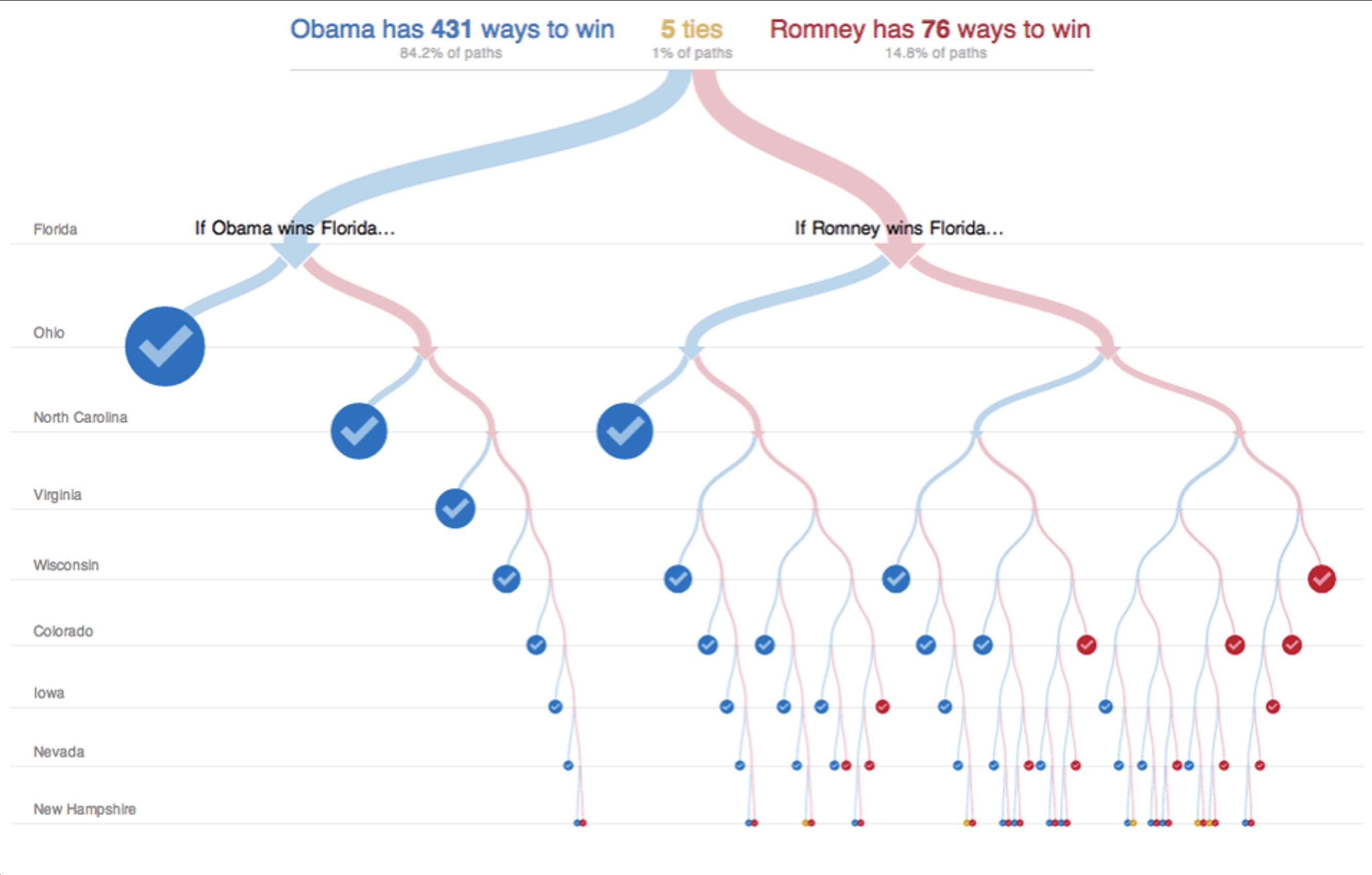
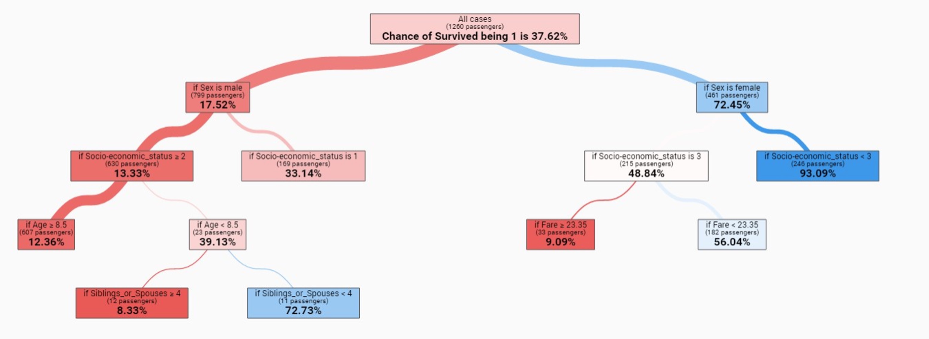
Special Trees: Decision Trees

Decision Tree: Each node = decision point

Two contexts:

1. Human decision-making (flowcharts, election scenarios)
2. Machine learning (learned classification models)

Why visualize: Interpretability, debugging, trust, bias detection

NYT Election Tree

ML Decision Tree

• NYT 512 Paths: 2012 election scenarios (9 swing states, 2⁹=512 outcomes)
• ML trees: Algorithm learns rules from data (split on attributes)
• Unlike neural nets, you can SEE the model! (Explainable AI)
• Used in medicine, finance, criminal justice (require transparency)

Treemaps

Space-filling approach for large hierarchies

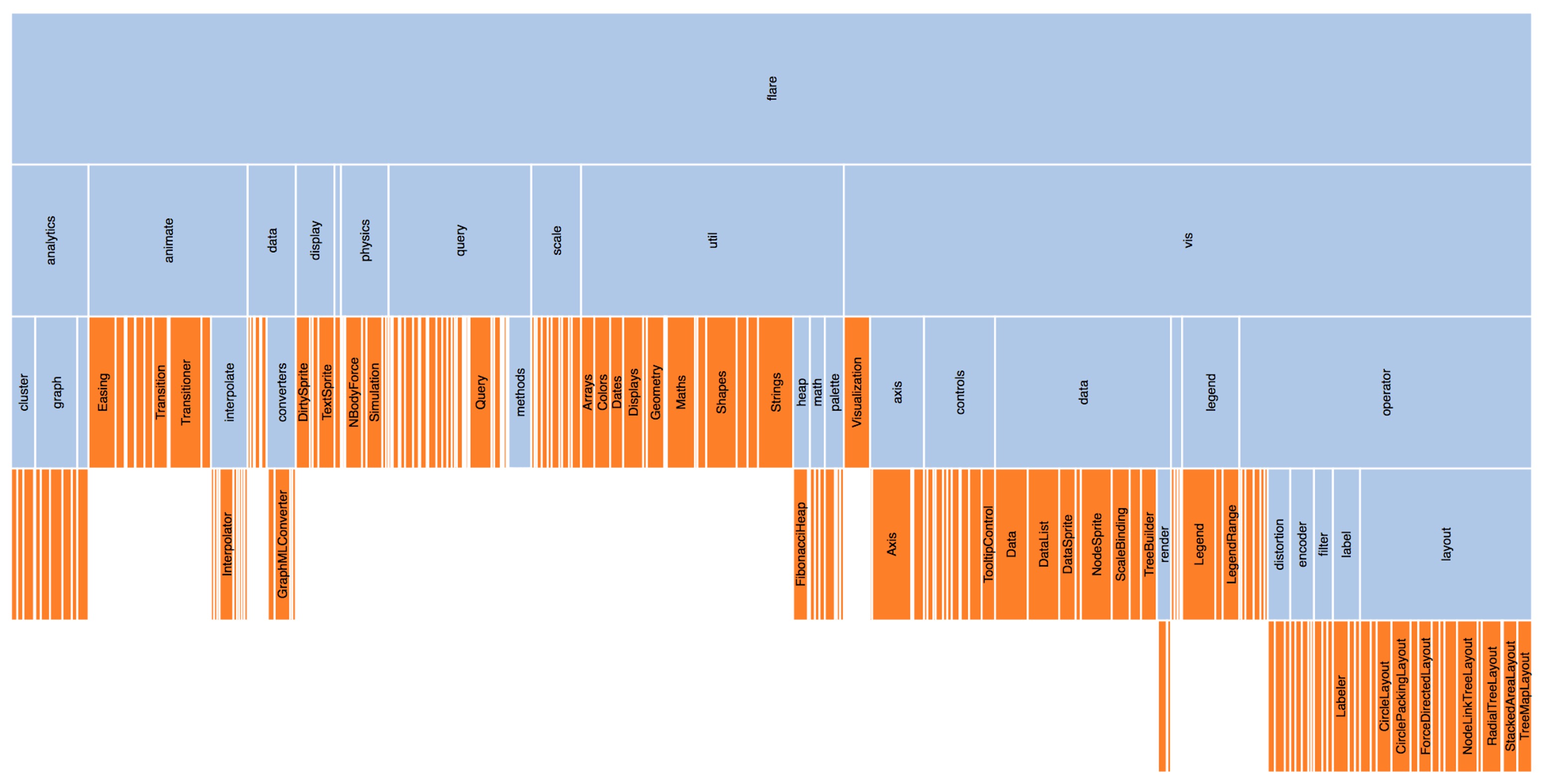
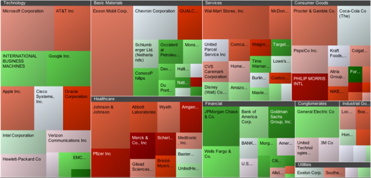
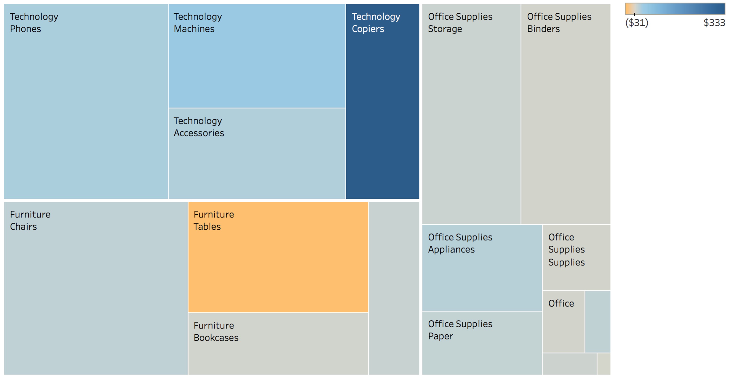
Treemaps: Origin & Encoding

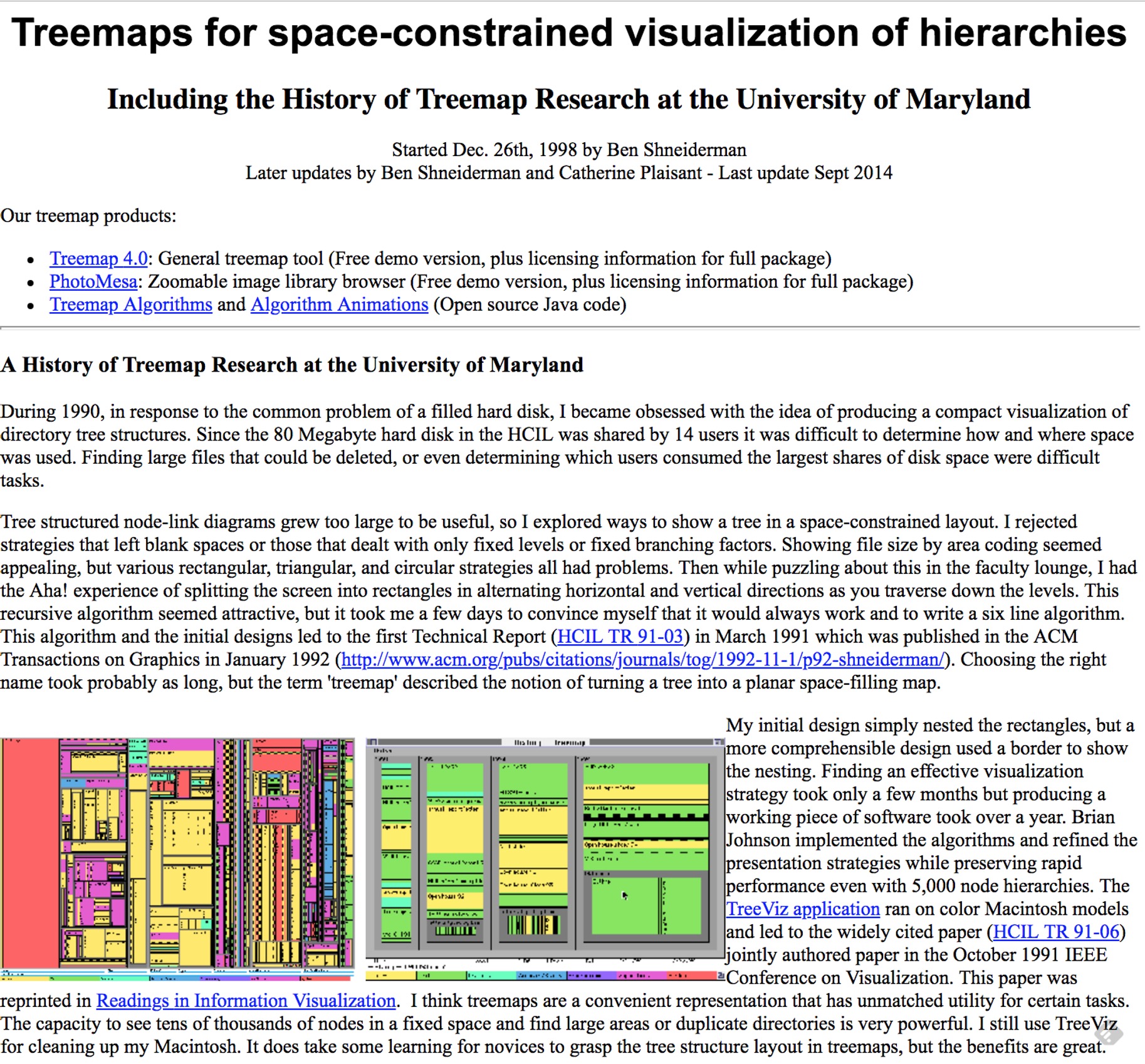
Origin (Ben Shneiderman, 1990): “My hard disk is full - what’s using space?”

Encoding:

• Area: Quantitative value (size, revenue, count)
• Color: Category OR secondary metric
• Nesting: Hierarchical structure

Key innovation: Shows BOTH hierarchy AND size

• Solving personal frustration → major innovation (5000+ citations)
• Area proportional to value, sum of children = parent
• Widely adopted: WinDirStat, DaisyDisk, Google Analytics, finance
• Can show 1000s of nodes (limited by screen resolution, not algorithm)

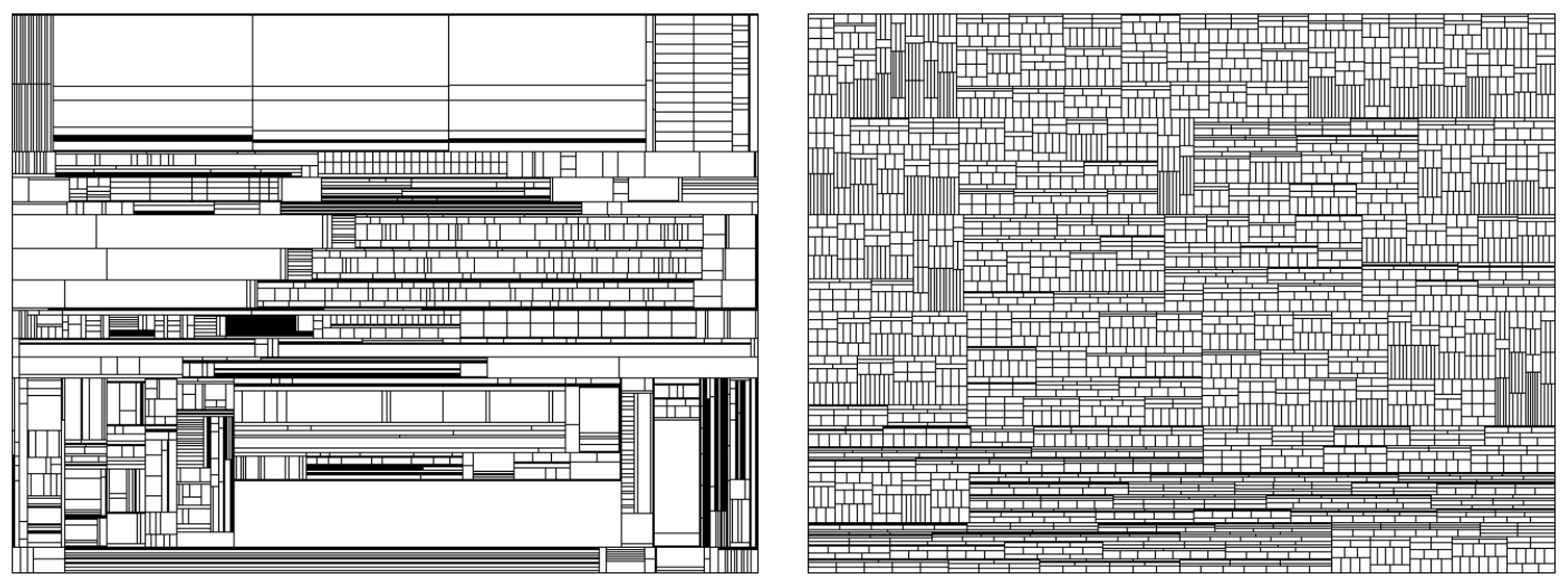
Treemap Algorithms: Squarified vs Slice-and-Dice

Problem: Slice-and-Dice creates thin rectangles (bad aspect ratios)

Solution: Squarified algorithm optimizes for square-like shapes

Trade-off: Squarified is more readable but less stable (layout changes with data updates)

Squarified (better readability)

Comparison

• Perceptual research: Squares easier to compare than elongated rectangles
• Squarified: Greedy algorithm, local optimization of aspect ratios
• Use squarified for single snapshots, ordered treemaps for comparisons over time

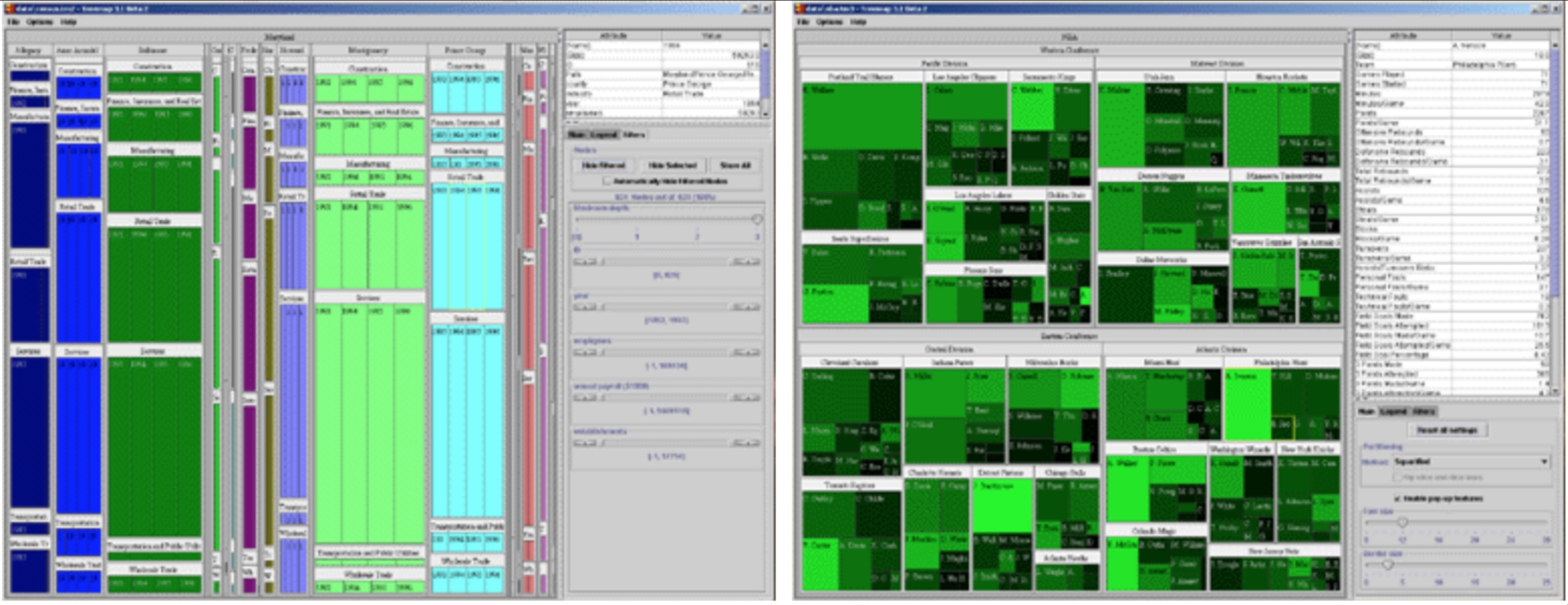
Treemap Examples

File Systems

Disk usage tools

Finance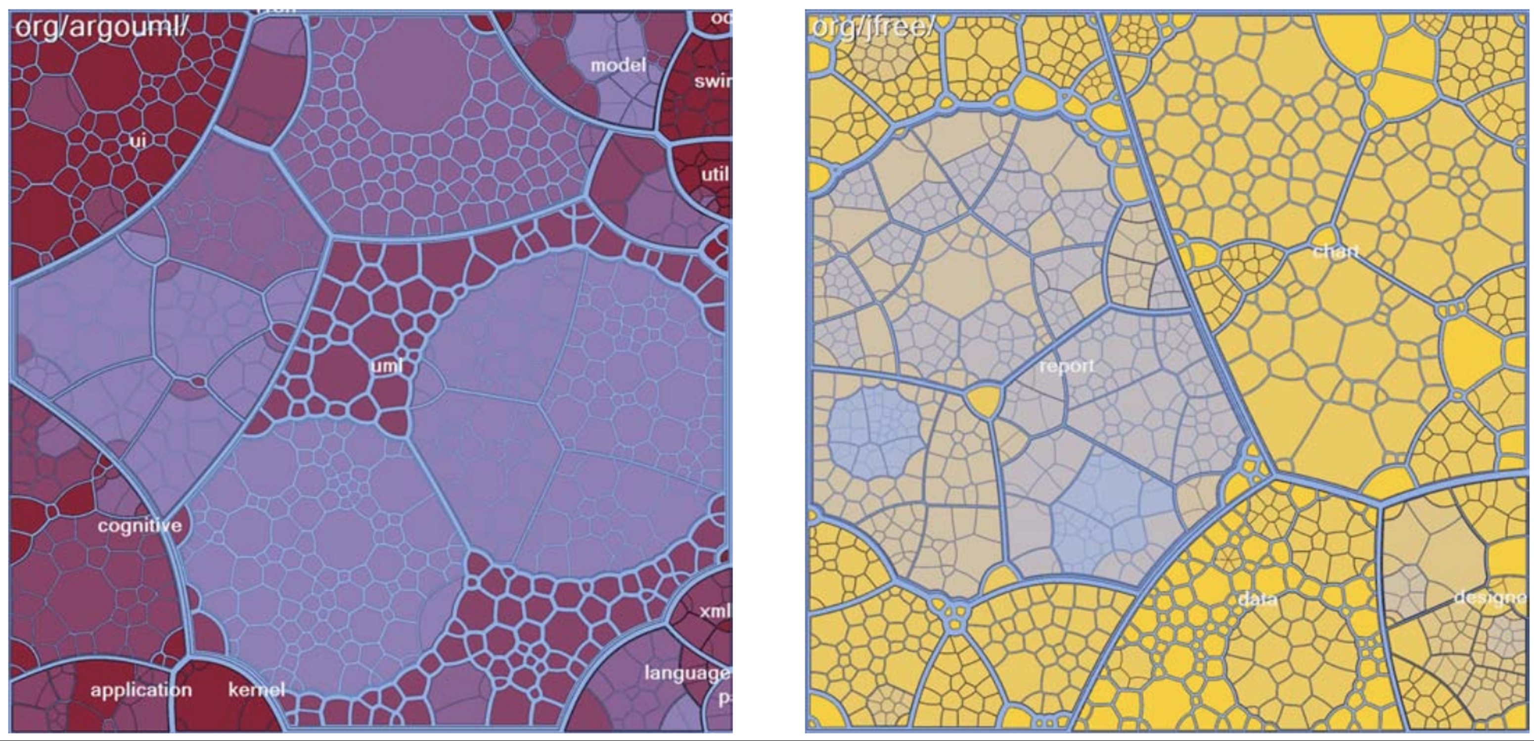

Stock market heat maps

Code Analysis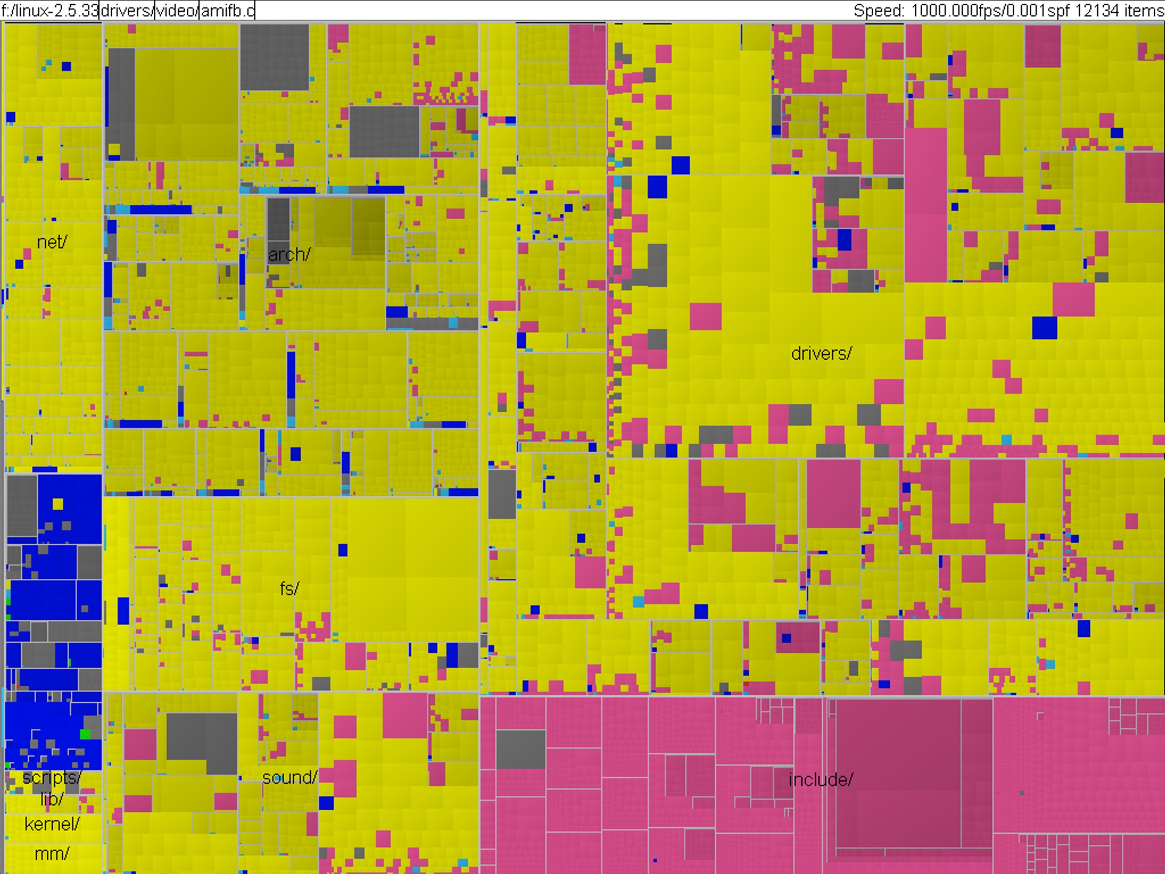

Linux kernel by file type

Applications: Business dashboards, news (Newsmap), analytics, sports

• Stock markets: Area=market cap, color=% change, grouped by sector
• Code: Area=file size, color=file type, reveals codebase structure
• Interaction: Zoom, hover for details, search/filter

Treemap Trade-offs

Advantages:

• ✓ Scalability (thousands of nodes)
• ✓ All nodes visible
• ✓ Encodes size + category
• ✓ Space-efficient

Disadvantages:

• ✗ Size less accurate than position
• ✗ Structure harder to see
• ✗ Layout algorithm affects readability

• When to use:
  • Large hierarchies (>100 nodes)
  • Quantitative data at leaves (size matters)
  • Need magnitude comparisons
• When NOT:
  • Small trees (<50 nodes) → node-link clearer
  • Structure more important than size
  • No meaningful quantitative attribute

Sunburst & Icicle Plots

Middle ground between node-link and treemaps:

• Sunburst: Radial (concentric rings)
• Icicle: Linear (horizontal bands)

Space efficiency: Treemap > Icicle > Sunburst Hierarchy perception: Icicle ≈ Sunburst > Treemap Familiarity: Treemap > Icicle > Sunburst

Sunburst

Icicle

• Use when both structure AND size matter
• Sunburst: Beautiful, angle=proportion, radius=depth
• Fixed height/width per level (less efficient than treemaps)
• Growing in popularity with interactive zoomable versions

Summary & Recommendations

Visualization Method Summary

Networks (General Graphs):

• Force-Directed: Unknown structure, exploration, <100 nodes
• Fixed Layout: Known groupings, spatial data, semantic positioning
• Matrix: Dense networks, analytical tasks, expert users

Trees (Hierarchies):

• Node-Link: Small trees (<100), structure focus, intuitive
• Treemaps: Large trees (1000s), size focus, space-efficient
• Sunburst/Icicle: Balance of structure + size, moderate depth

Key principle: No single “best” method - depends on data, task, audience

• Data size drives choice (sparse vs dense, small vs large)
• Task matters (structure vs values, paths vs clusters, overview vs details)
• Audience matters (experts vs general public, static vs interactive)
• Often use multiple views with linking

Design Guidelines & Trade-offs

Key dimensions to consider:

1. Clutter: How crowded?
2. Scalability: How many nodes/edges?
3. Structure visibility: How clear is topology?
4. Familiarity: How intuitive for audience?
5. Reordering needs: Preprocessing required?

Decision process: Try multiple approaches → prototype → user test → iterate

• No perfect visualization - all involve trade-offs
• Clutter: Node-link high (dense graphs), Matrix low
• Scalability: Node-link ~100, Matrix ~1000, Treemap ~10,000
• Structure: Force-directed high, Fixed low (unless meaningful)
• Best practice: Prototype multiple, use linked views, provide interaction

Programming Exercises (suggestion!)

Create variants of each technique:

1. Force-directed layout: Implement algorithm OR use D3.js, experiment with encodings
2. Circular/chord diagram: Fixed layout with edge bundling
3. Node-link tree: Top-down OR radial, with collapse/expand
4. Treemap: Squarified algorithm with zoom/drill-down

Explore:

• Visual encodings (size, color, thickness)
• Interaction (zoom, filter, details-on-demand)
• Real datasets (social, citations, file systems, hierarchical clustering)

Tools: D3.js, Gephi, Cytoscape, NetworkX (Python), igraph (R)

• Encourage: Implement from scratch (learn algorithms) AND use libraries (practical)
• Datasets available: Course website, Gephi sample data, D3 examples
• Focus on design decisions (encodings, interaction, layout parameters)

Resources & References

Essential readings:

• Shirley Wu: Understanding the Force
• Holten (2006): Hierarchical Edge Bundling - IEEE TVCG
• Shneiderman (1992): Tree Visualization with Tree-maps - ACM TOG
• Bruls et al. (2000): Squarified Treemaps - Springer

Advanced topics: Motif simplification (Dunne & Shneiderman), semantic substrates, time-varying networks, multilayer networks

Interactive examples: Observable (D3.js), Gephi tutorials, Graph visualization survey papers

• Shirley Wu’s article is THE best force-directed tutorial
• Holten & Shneiderman papers are foundational (must-reads)
• Observable has live, editable examples (great for learning)
• Encourage exploration of tools (Gephi for analysis, D3 for custom viz)

Thank You!

Next class: Week 14 - Final Project Presentations

Questions?

• Key takeaways:
  • Two paradigms: Node-link vs Matrix
  • Trees enable specialized techniques
  • Always consider: Data, Task, Audience
  • Prototype multiple approaches
  • Interaction overcomes static limitations
• Office hours: Available for project help
• Reminder: Programming assignments + readings