Black-box Model Interpretation

CS-GY 9223 - Fall 2025

Claudio Silva

NYU Tandon School of Engineering

2025-10-06

Black Box Model Assessment

Agenda

Goal: Study Model Agnostic Interpretability Methods. These should help to explain any type of ML Models.

1. Partial Dependence Plot (PDP)

2. Local Interpretable Model-agnostic Explanations (LIME)

3. SHAP (SHapley Additive exPlanations)

4. Comparative Analysis and Trade-offs

Acknowledgments:

Materials adapted from:

• Molnar, C. (2024). Interpretable Machine Learning
• Molnar, C. (2024). Interpreting Machine Learning Models With SHAP

Today we transition from white-box (interpretable) models to black-box explanation methods. These techniques work with ANY machine learning model - neural networks, ensemble methods, etc. The key distinction: white-box models are inherently interpretable, while black-box methods provide post-hoc explanations. We’ll cover three major approaches: PDPs for global feature effects, LIME for local instance explanations, and SHAP for theoretically-grounded feature attribution. Each has different trade-offs between computational cost, interpretability, and theoretical guarantees. Significant portions of this lecture are adapted from Christoph Molnar’s excellent books on interpretable machine learning and SHAP.

Bike Rentals (Regression)

This dataset contains daily counts of rented bicycles from the bicycle rental company Capital-Bikeshare in Washington D.C., along with weather and seasonal information. The goal is to predict how many bikes will be rented depending on the weather and the day. The data can be downloaded from the UCI Machine Learning Repository.

Here is the list of features used in Molnar’s book:

• Count of bicycles including both casual and registered users. The count is used as the target in the regression task.
• The season, either spring, summer, fall or winter.
• Indicator whether the day was a holiday or not.
• The year, either 2011 or 2012.
• Number of days since the 01.01.2011 (the first day in the dataset). This feature was introduced to take account of the trend over time.
• Indicator whether the day was a working day or weekend.
• The weather situation on that day. One of: clear, few clouds, partly cloudy, cloudy mist + clouds, mist + broken clouds, mist + few clouds, mist light snow, light rain + thunderstorm + scattered clouds, light rain + scattered clouds heavy rain + ice pallets + thunderstorm + mist, snow + mist
• Temperature in degrees Celsius.
• Relative humidity in percent (0 to 100).
• Wind speed in km per hour.

Partial Dependence Plot (PDP)

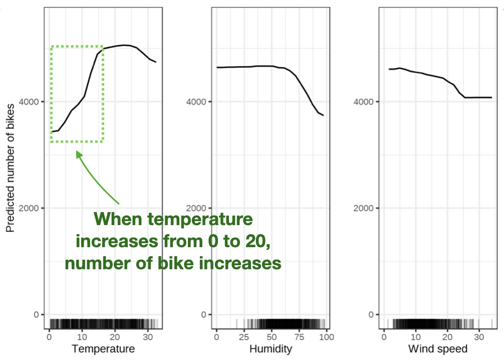
Shows the marginal effect one or two features have on the predicted outcome of a machine learning model (J. H. Friedman 2001).

1D PDP: Line plot showing effect of single feature

2D PDP (Interaction Plots):

For two features, PDP generates a heatmap showing interactions.

🟦🟦🟨🟧🟧
🟦🟦🟨🟧🟧
🟩🟩🟨🟨🟨
🟩🟩🟨🟨🟨

Complex contours = strong feature interaction

PDPs are one of the oldest and most intuitive model-agnostic interpretation methods. The key idea: marginalize over all other features to isolate the effect of one (or two) features on the prediction. Here we see bike rentals vs temperature - notice the non-linear relationship with a sweet spot around 20-25°C. The visualization immediately reveals this pattern that might be hidden in model coefficients. For two features, PDP generates a 2D plot (heatmap) showing interactions - the more complex the contour lines, the stronger the interaction between features. For example, a 2D PDP of temperature × humidity might show that high temperature increases rentals only when humidity is low. PDPs answer: “On average, how does changing this feature affect predictions?”

PDP Visualization: Interpreting Feature Effects

1. Monotonic/Linear

↗
  ↗
    ↗

Straight diagonal line

↑ Feature → ↑ Prediction

Feature has consistent positive (or negative) effect

2. Non-linear/Sweet Spot

   ╱‾╲
  ╱    ╲
 ╱      ╲

Curve peaks and drops

Optimal range exists

(like temperature example)

3. Flat Line

━━━━━━━

Horizontal line

No marginal effect

Feature is globally unimportant

The key visual takeaway is the slope and shape of the line. The slope indicates the marginal effect. A flat line is a visually clear indicator of a globally unimportant feature. Contrast the flat line with the non-linear “sweet spot” of the temperature plot from the previous slide. When reviewing PDPs, look for: (1) Direction of effect (up/down), (2) Linearity vs non-linearity, (3) Interaction points where the effect changes dramatically.

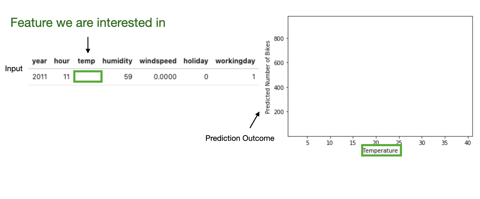
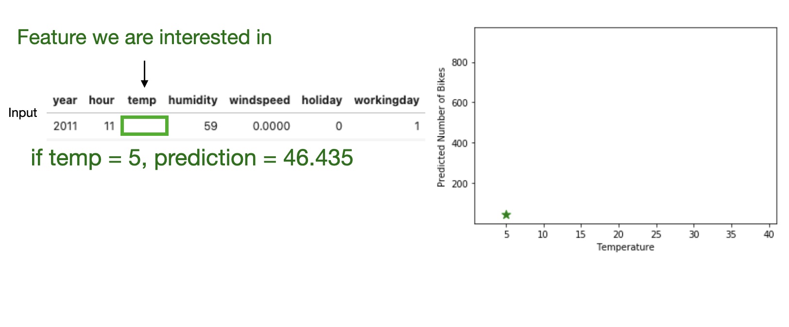
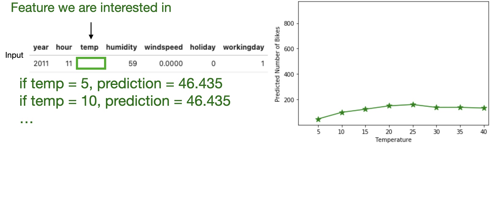
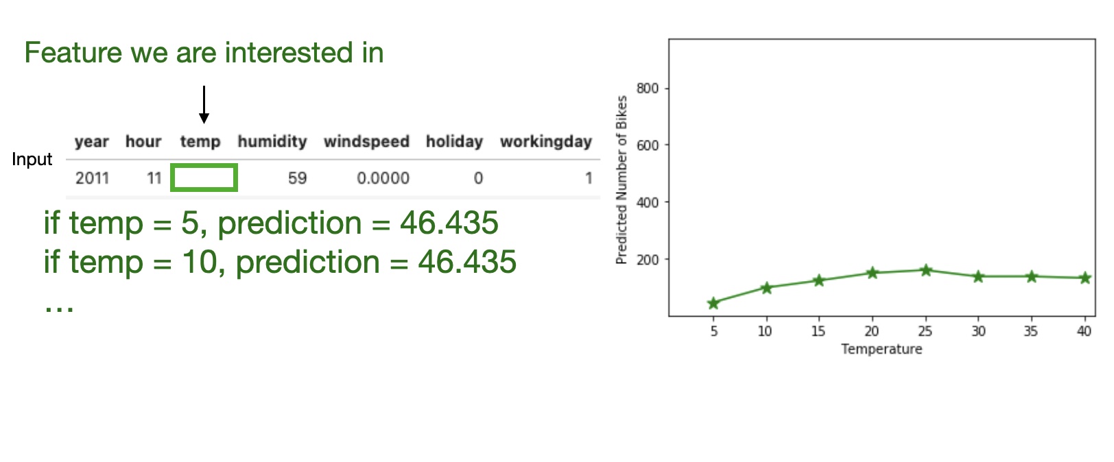
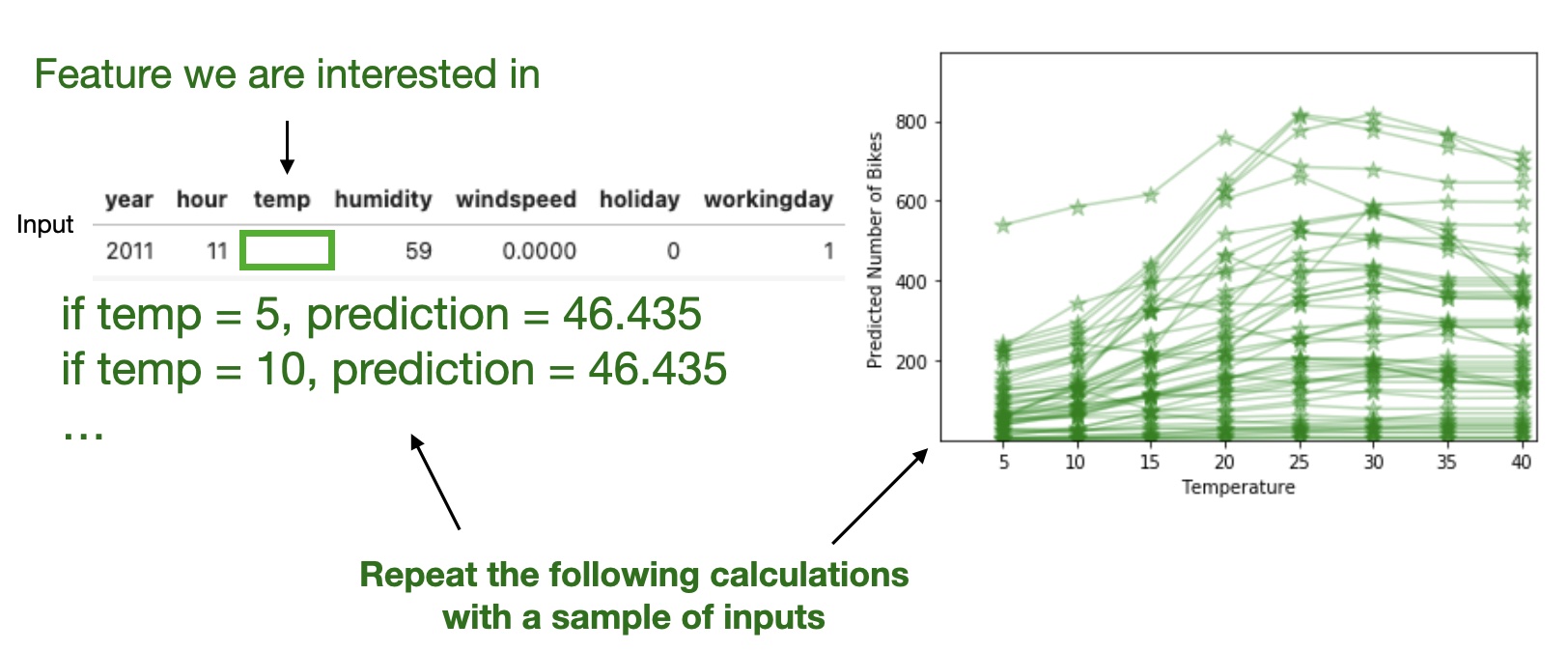
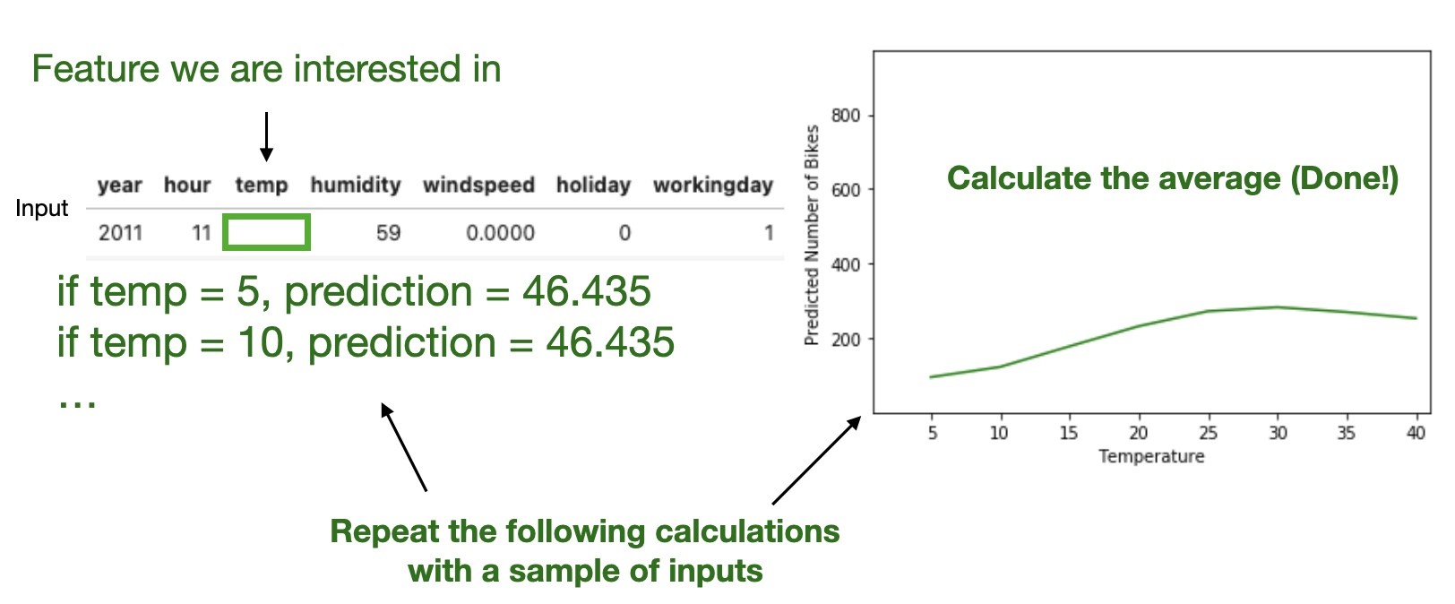
Partial Dependence Plot (PDP)

High level idea: marginalizing the machine learning model output over the distributions of the all other features to show the relationship between the feature we are interested in and the predicted outcome.

This animation shows the PDP computation process step by step. For each value of our feature of interest, we: (1) Replace that feature with a fixed value across ALL data points, (2) Get predictions for all those modified instances, (3) Average those predictions, (4) Repeat for different feature values. The result is a curve showing the average effect. Notice how we’re effectively “scanning” through the feature space while averaging out the effects of all other features. This is powerful because it works with any black-box model.

While the animation shows the calculation (marginalizing/averaging), remind students that the resulting simple 2D line plot is the visualization product we interpret. The computational complexity is hidden from the end user - they only see the clean, interpretable curve that reveals the feature’s marginal effect.

PDP: Code Example with scikit-learn

Dataset: California Housing - median house value prediction (8 features)

from sklearn.datasets import fetch_california_housing
from sklearn.ensemble import GradientBoostingRegressor
from sklearn.inspection import PartialDependenceDisplay
import matplotlib.pyplot as plt

# Load California housing dataset
# Features: median income, house age, average rooms, etc.
housing = fetch_california_housing()
X, y = housing.data, housing.target

# Train a gradient boosting regressor
model = GradientBoostingRegressor(
    n_estimators=100,
    max_depth=4,
    learning_rate=0.1,
    random_state=0
).fit(X, y)

# Create PDPs for: MedInc (0), HouseAge (1), and their interaction
# MedInc = median income, HouseAge = median house age
features = [0, 1, (0, 1)]
display = PartialDependenceDisplay.from_estimator(
    model, X, features, feature_names=housing.feature_names
)

This example shows how simple it is to compute PDPs in practice using scikit-learn. The PartialDependenceDisplay.from_estimator() method handles all the computation automatically: (1) It marginalizes over the training data, (2) Computes predictions for all feature values, (3) Averages the results, (4) Creates the visualization. Note that you can plot individual features [0, 1] or interactions [(0, 1)] which show how two features jointly affect predictions. The interaction plot is a 2D heatmap instead of a line plot. This high-level API abstracts away the complexity we saw in the animation, making PDPs accessible for practitioners.

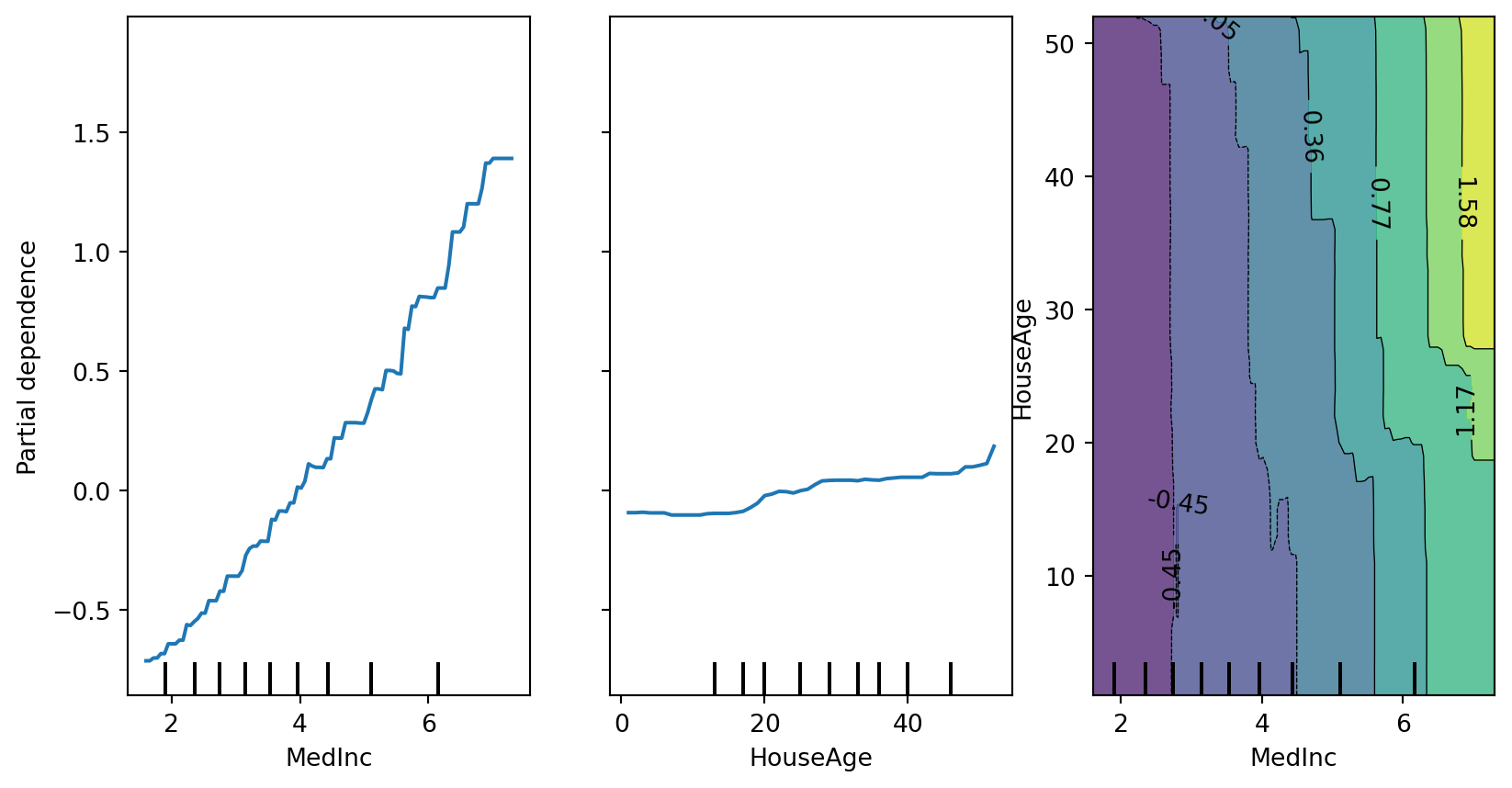
PDP: Output Visualization

Interpretation:

• Left (MedInc): Strong positive monotonic relationship - higher median income → higher house prices (as expected)
• Middle (HouseAge): Non-monotonic effect - newer and very old houses have lower values, middle-aged houses peak
• Right (Interaction): Shows how income and age combine - high income dominates regardless of age (vertical gradient)

The California Housing dataset provides much clearer, more interpretable patterns: (1) MedInc (Median Income): Shows a strong, near-linear positive relationship - as median income increases, predicted house values increase consistently. This makes intuitive sense and demonstrates a clear monotonic effect. (2) HouseAge: Reveals a non-monotonic pattern with a peak for middle-aged houses (around 20-30 years). Very new houses might lack established neighborhoods, while very old houses may need renovation. This is the kind of “sweet spot” pattern we discussed earlier. (3) Interaction plot: The 2D heatmap shows that median income has a dominant effect (notice the strong vertical color gradient), while house age modulates this effect more subtly. The interaction reveals that high-income areas command high prices regardless of house age. These diverse patterns demonstrate why PDPs are valuable for understanding feature effects.

Partial Dependence Plot (PDP)

Pros

• Intuitive
• Interpretation is clear
• Easy to implement

Cons

• Assume independence among features
• Can only show few features
• Hidden heterogeneous effects from averaging

From Global to Local: Bridging PDP to LIME

PDP’s Limitation: Averaging Hides Individual Differences

The Problem:

PDP shows the average effect across all instances.

But what if the effect differs between: - Cold days vs. warm days? - New customers vs. loyal customers? - Low-income vs. high-income applicants?

PDP cannot tell you!

The Solution:

Move from global to local explanations.

Instead of asking: > “How does temperature affect rentals on average?”

Ask: > “Why did the model predict this specific value for this particular day?”

→ Enter LIME

This slide bridges the conceptual gap between PDP and LIME. PDP’s key limitation - “hidden heterogeneous effects from averaging” - means we lose important information about how features affect different types of instances differently. For example, temperature might increase bike rentals on sunny days but decrease them on rainy days, and PDP would just show the average. This motivates the need for local explanations that focus on individual instances. LIME addresses this by building interpretable surrogate models around specific predictions, allowing us to understand “why THIS prediction for THIS instance?” rather than just global averages.

Local Interpretable Model-agnostic Explanations (LIME)

Training local surrogate models to explain individual predictions

LIME represents a paradigm shift from global to local explanations. The key insight: even if the global decision boundary is complex (left image shows a highly non-linear boundary), we can approximate it LOCALLY with a simple linear model. Think of it like approximating a curve with a tangent line - it only works near the point of tangency. The title “Why Should I Trust You?” captures the motivation: users need to understand individual predictions to build trust. LIME became hugely influential because it’s model-agnostic, produces human-interpretable explanations, and works for any data type (tabular, text, images).

Training local surrogate models to explain individual predictions

The idea is quite intuitive. First, forget about the training data and imagine you only have the black box model where you can input data points and get the predictions of the model. You can probe the box as often as you want. Your goal is to understand why the machine learning model made a certain prediction. LIME tests what happens to the predictions when you give variations of your data into the machine learning model.

LIME generates a new dataset consisting of perturbed samples and the corresponding predictions of the black box model.

On this new dataset LIME then trains an interpretable model, which is weighted by the proximity of the sampled instances to the instance of interest. The interpretable model can be anything from the interpretable models chapter, for example Lasso or a decision tree. The learned model should be a good approximation of the machine learning model predictions locally, but it does not have to be a good global approximation. This kind of accuracy is also called local fidelity.

Mathematically, local surrogate models with interpretability constraint can be expressed as follows:

\[\text{explanation}(x) = \arg\min_{g \in G} L(f, g, \pi_x) + \Omega(g)\]

Local Interpretable Model-agnostic Explanations (LIME)

Algorithm

1. Pick an input that you want an explanation for.
2. Sample the neighbors of the selected input (i.e. perturbation).
3. Train a linear classifier on the neighbors.
4. The weights on the linear classifier is the explanation.

Local Interpretable Model-agnostic Explanations (LIME)

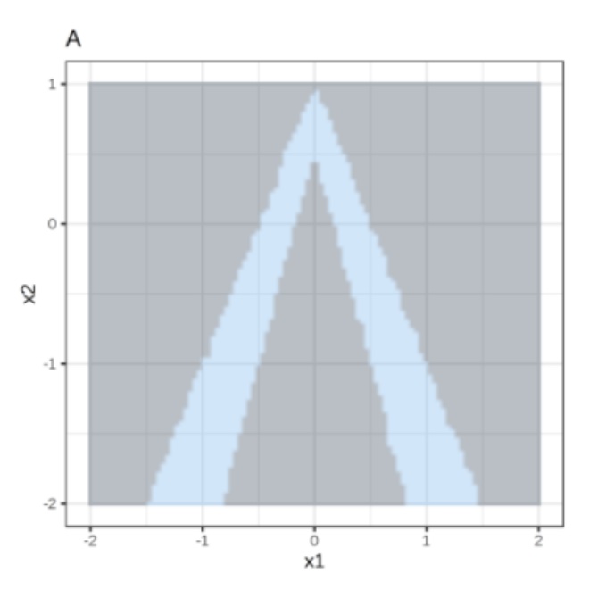
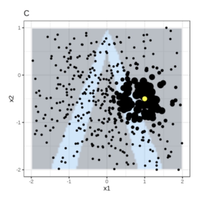
Random forest predictions given features x1 and x2.

Predicted classes: 1 (dark) or 0 (light).

Local Interpretable Model-agnostic Explanations (LIME)

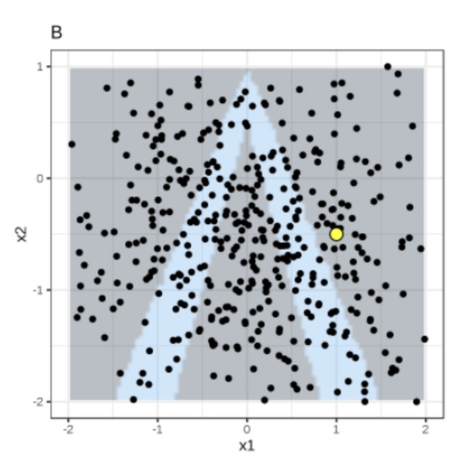
Instance of interest (big yellow dot) and data sampled from a normal distribution (small dots).

Local Interpretable Model-agnostic Explanations (LIME)

Assign higher weight to points near the instance of interest. I.e., \(weight(p) = \sqrt{\frac{e^{-d^2}}{w^2}}\) where \(d\) is the distance between \(p\) and the instantce of interest, and \(w\) is the kernel width (self-defined).

Local Interpretable Model-agnostic Explanations (LIME)

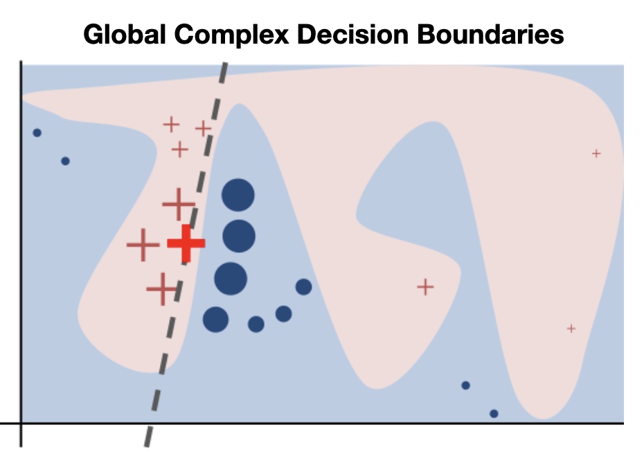
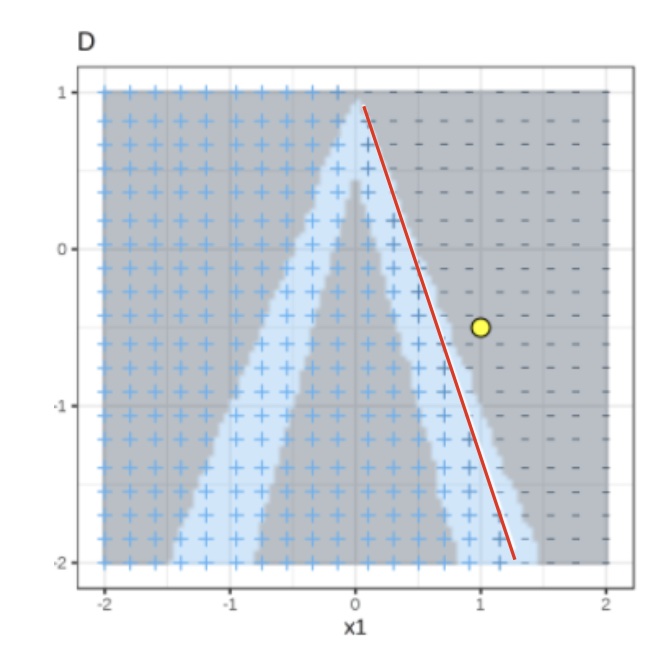
Use both the samples and sample weights to train a linear classifier.

Signs of the grid show the classifications of the locally learned model from the weighted samples. The red line marks the decision boundary (P(class=1) = 0.5).

The official implementation uses a Ridge Classifier as the linear model for explanation.

Training local surrogate models to explain individual predictions

\(s_i\) = sample weight, \(\lambda\) = regularization term

Ridge Classifier

\[minimize \sum_{i=1}^{M} s_i(y_i - \hat{y}_i)^2\]

\[= \sum_{i=1}^{M} s_i(y_i - \sum_{j=0}^{p} w_j \times x_{ij})^2 + \lambda \sum_{j=0}^{p} w_j^2\]

\(w_j\) = trained weight to explain the importance of feature j

The higher the \(\lambda\), the more sparse the \(w\) (more zeros) will become.

LIME Visualization: Bar Charts for Local Explanations

Primary LIME Output: Sparse Bar Charts

Case 1: High Rental Day Prediction: ABOVE Trend

▬▬▬▬▬▬▬▬▬▬ Temp > 20°C

▬▬▬▬▬▬▬ Windspeed Low

▬▬▬ Holiday = False

✓ Warm temperature strongly supports high rentals ✓ Low wind moderately supports ✗ Non-holiday slightly opposes

Case 2: Low Rental Day Prediction: BELOW Trend

▬▬▬▬▬▬▬▬▬▬▬▬ Weather: Rain

▬▬▬▬▬▬▬▬ Temp < 5°C

▬▬ Weekday = True

✗ Rain strongly opposes high rentals ✗ Cold temperature opposes ✓ Weekday weakly supports

Emphasize the visualization: Color (Green supports the prediction, Red opposes it), Length of Bar (magnitude of influence), and Sparsity (only a few features are shown—this makes it easy for a non-expert to trust). The bar chart is the key deliverable of LIME - it provides a contrastive explanation showing which features push toward vs away from the prediction. Compare the two cases: Case 1 is dominated by green (supporting features), while Case 2 is dominated by red (opposing features). This visual contrast makes the explanation immediately understandable.

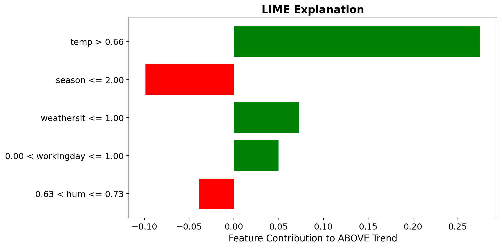
Local Surrogate (LIME): Bike Rental Example

Task: Predict if bike rentals will be above or below trend

High Rental Day

Prediction: {python} f”{pred_high[1]:.2f}“ probability ABOVE trend

✓ High temperature strongly supports
✓ Good weather condition supports

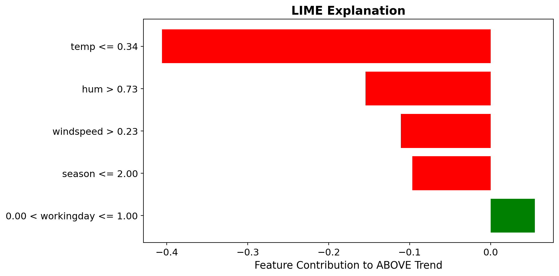
Low Rental Day

Prediction: {python} f”{pred_low[0]:.2f}“ probability BELOW trend

✗ Bad weather strongly opposes
✗ Low temperature opposes

This slide shows actual LIME explanations for bike rental predictions. The bar charts display feature contributions - green bars indicate features supporting the prediction, orange/red bars indicate features opposing it. Notice how the high rental day is dominated by positive contributions (warm temp, good weather), while the low rental day is dominated by negative contributions (bad weather, cold temp). The model predictions are shown at the top - one instance has high probability of being ABOVE trend, the other BELOW trend. This is exactly the kind of local explanation LIME provides - understanding which features matter most for each specific prediction.

Local Surrogate (LIME)

Training local surrogate models to explain individual predictions

This figure demonstrates LIME’s model-agnostic nature applied to image classification with Google’s Inception neural network. The key adaptation for images is using superpixels (coherent image regions) as interpretable features instead of individual pixels. Notice how LIME provides instance-specific explanations: when explaining “Electric guitar” (p=0.32), it highlights the guitar; when explaining “Acoustic guitar” (p=0.24), it highlights acoustic features; when explaining “Labrador” (p=0.21), it highlights the dog’s face. This shows that different predictions for the same image get different explanations - LIME adapts to explain what matters for each specific prediction. The gray regions are turned off (superpixels not contributing to that prediction), while colored regions are what the local linear model identifies as most important.

Local Surrogate (LIME)

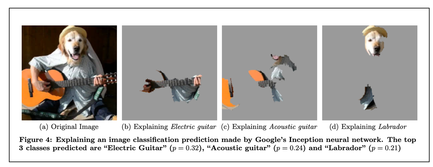
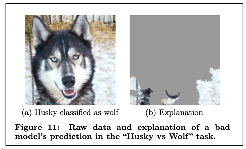
Raw data and explanation of a bad model’s prediction in the “Husky vs Wolf” task

This is one of the most famous examples from the LIME paper, demonstrating its value for model debugging. A husky is incorrectly classified as a wolf. The LIME explanation reveals why: the model is focusing on the background snow rather than the animal’s features. This exposes a serious flaw - the model learned a spurious correlation between wolves and snowy backgrounds in the training data, rather than learning actual wolf features. Without LIME, this model might have seemed accurate on test data, but would fail catastrophically in the real world when encountering wolves without snow or huskies with snow. This illustrates LIME’s critical role in building trust and identifying when NOT to trust a model. The explanation shows which superpixels the model is using - and in this case, it’s using the wrong ones.

LIME: Code Example

Dataset: California Housing (same model as PDP example)

import lime
import lime.lime_tabular
import numpy as np

# Reload California Housing data for this example
housing = fetch_california_housing()
X_housing, y_housing = housing.data, housing.target

# Retrain model on California Housing
model = GradientBoostingRegressor(
    n_estimators=100,
    max_depth=4,
    learning_rate=0.1,
    random_state=0
).fit(X_housing, y_housing)

# Create LIME explainer using training data
explainer = lime.lime_tabular.LimeTabularExplainer(
    training_data=X_housing,
    feature_names=housing.feature_names,
    mode='regression',
    random_state=0
)

# Select an instance to explain (e.g., instance 0)
instance_idx = 0
instance = X_housing[instance_idx]

# Generate explanation for this instance
# predict_fn should return predictions
exp = explainer.explain_instance(
    instance,
    model.predict,
    num_features=5  # Show top 5 features
)

LIME provides local explanations by training a simple interpretable model around a specific instance. The LimeTabularExplainer is initialized with the training data to understand feature distributions. The key parameter is num_features which controls sparsity - we only show the top 5 most important features for this prediction. Unlike PDP which gives global effects, LIME explains why the model made this specific prediction for this specific instance. The predict function is passed to LIME so it can probe the model with perturbed versions of the instance.

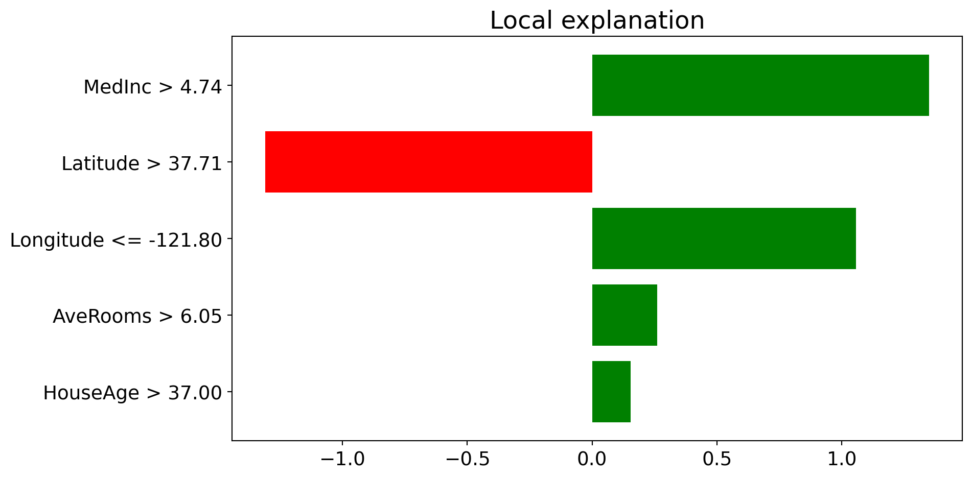
LIME: Output Visualization

Explanation for Instance 0:

Predicted value: 4.29 (in units of $100k)

The bar chart shows which features push the prediction higher (positive) or lower (negative) for this specific house.

The output shows a horizontal bar chart with the most important features for this specific prediction. Positive bars (pointing right) indicate features that increase the predicted house value, while negative bars (pointing left) decrease it. The length of each bar represents the magnitude of the feature’s contribution. Notice this is a LOCAL explanation - it only applies to this one house. If we explained a different house, we’d likely get different important features. This is the key difference from PDP which shows global average effects. The sparse representation (only 5 features) makes it easy for users to understand and trust the prediction.

Local Interpretable Model-agnostic Explanations (LIME)

Pros

• Explanations are short (= selective) and possibly contrastive.
  • we can control the sparsity of weight coefficients in the regressions method.
• Very easy to use.

Cons

• Unstable results due to sampling.
• Hard to weight similar neighbors in a high dimensional dataset.
• Many parameters for data scientists to hide biases.

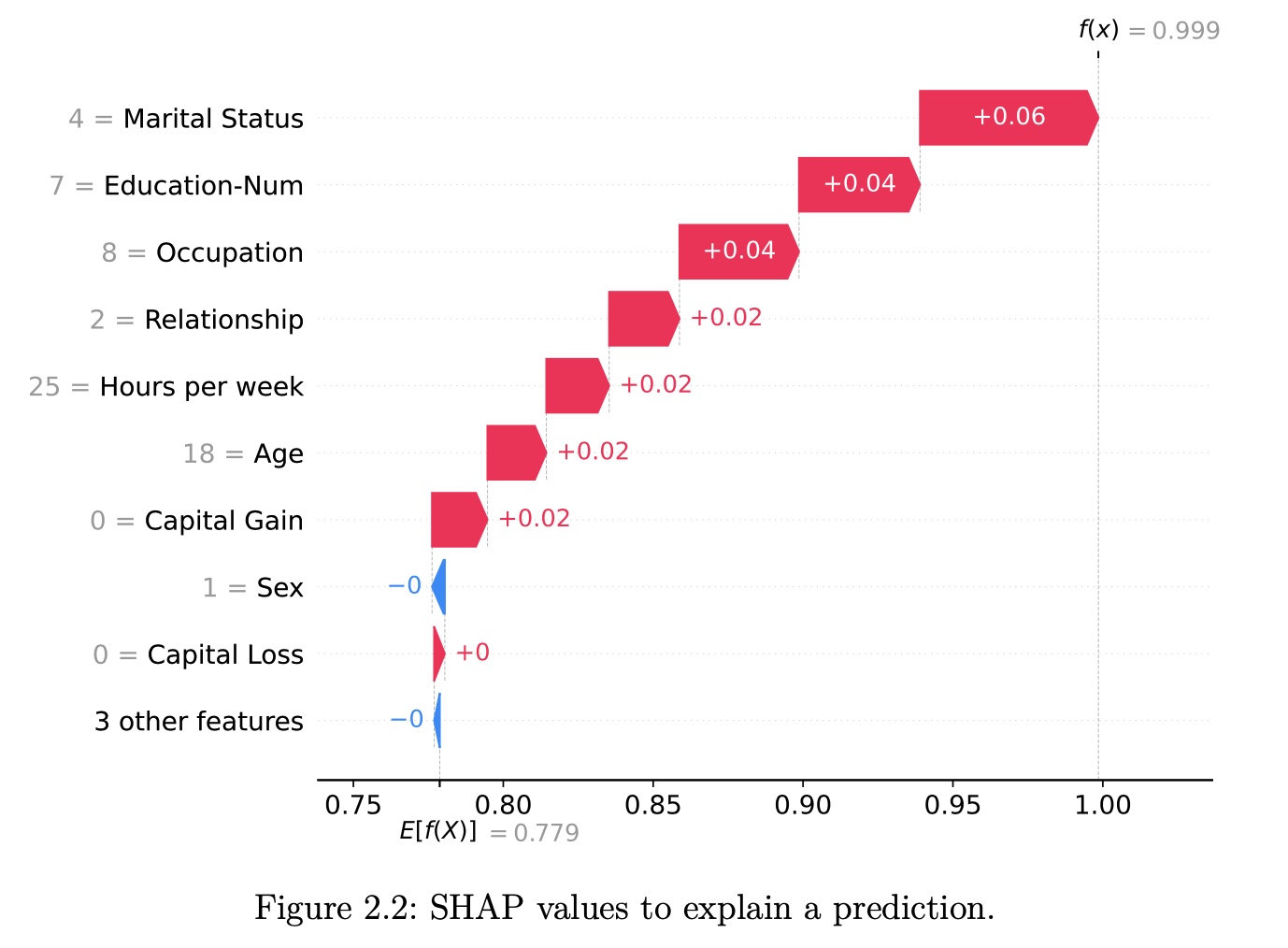
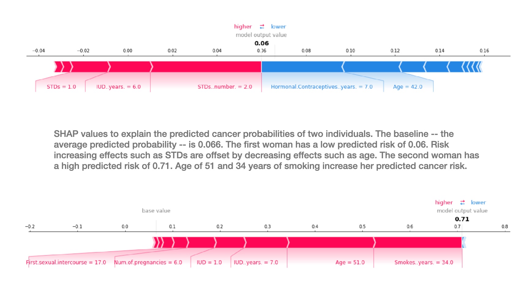
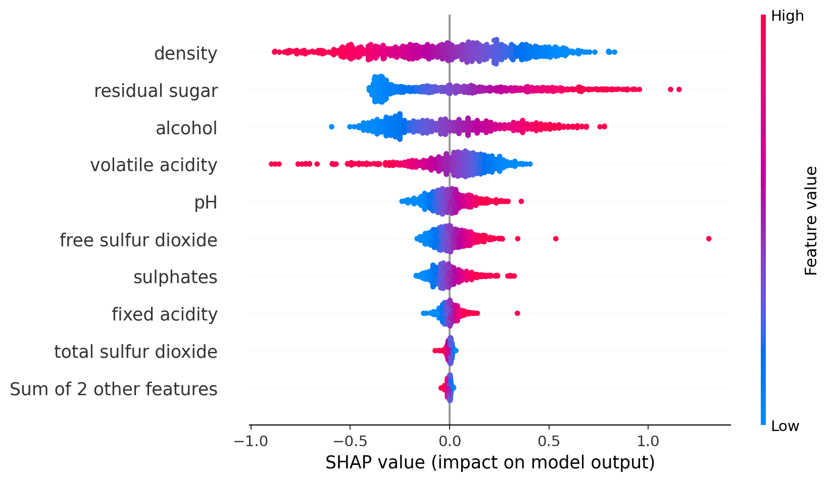
SHAP (SHapley Additive exPlanations)

SHAP (Lundberg and Lee 2017a) is a game-theory-inspired method created to explain predictions made by machine learning models. SHAP generates one value per input feature (also known as SHAP values) that indicates how the feature contributes to the prediction of the specified data point.

SHAP brings rigorous game theory to ML interpretability. The key innovation: apply Shapley values from cooperative game theory to feature attribution. This provides a principled answer to “how much did each feature contribute?” with mathematical guarantees (efficiency, symmetry, dummy, additivity axioms). SHAP unified several existing methods under one framework. The image shows a typical SHAP force plot - red pushes prediction higher, blue pushes lower. Unlike LIME which is heuristic, SHAP has strong theoretical foundations. Trade-off: computational cost is higher, but you get provably fair attributions.

A Short History of Shapley Values and SHAP

Three key milestones:

• 1953: The introduction of Shapley values in game theory
• 2010: The initial steps toward applying Shapley values in machine learning
• 2017: The advent of SHAP, a turning point in machine learning

Lloyd Shapley’s Pursuit of Fairness (1953)

Lloyd Shapley - “The greatest game theorist of all time”

• PhD at Princeton (post-WWII): “Additive and Non-Additive Set Functions”
• 1953 paper: “A Value for n-Person Games”
• 2012 Nobel Prize in Economics (with Alvin Roth) for work in market design and matching theory

The Problem: How to fairly divide payouts among players who contribute differently to a cooperative game?

The Solution: Shapley values provide a mathematical method for fair distribution based on marginal contributions

Applications of Shapley values:

• Political science
• Economics
• Computer science
• Dividing profits among shareholders
• Allocating costs among collaborators
• Assigning credit in research projects

Key insight: By 1953, Shapley values were well-established in game theory, but machine learning was still in its infancy.

Early Days in Machine Learning (2010)

2010: Erik Štrumbelj and Igor Kononenko propose using Shapley values for ML

• Paper: “An efficient explanation of individual classifications using game theory”
• 2014 follow-up: Further methodology development

Why didn’t it gain immediate traction?

❌ Barriers to adoption:

1. Explainable AI/Interpretable ML not widely recognized yet
2. No code released with the papers
3. Estimation method too slow for images/text
4. Limited awareness outside specialized communities

✅ What was needed:

1. Growing demand for interpretability
2. Open-source implementation
3. Faster computation methods
4. High-profile publication venue
5. Integration with popular ML frameworks

The SHAP Cambrian Explosion (2017)

2016: LIME paper catalyzes the field

Ribeiro et al. introduce Local Interpretable Model-Agnostic Explanations → growing interest in model interpretability

2017: Lundberg and Lee publish SHAP at NeurIPS

“A Unified Approach to Interpreting Model Predictions”

Key contributions beyond 2010 work:

1. Kernel SHAP: New estimation method using weighted linear regression
2. Unification framework: Connected SHAP to LIME, DeepLIFT, and Layer-Wise Relevance Propagation
3. Open-source shap package: Wide range of features and plotting capabilities
4. High-profile venue: Published at major ML conference (NIPS/NeurIPS)

Why SHAP Gained Popularity

Critical success factors:

✓ Published at prestigious venue (NeurIPS) ✓ Pioneering work in rapidly growing field ✓ Open-source Python package - enabled integration ✓ Ongoing development by original authors ✓ Strong community contributions ✓ Comprehensive visualization tools

2020 breakthrough: TreeSHAP

• Efficient computation for tree-based models
• Enabled SHAP for state-of-the-art models
• Made global interpretations possible

Naming conventions:

• Shapley values: Original game theory method (1953)
• SHAP: Application to machine learning (2017)
• SHAP values: Resulting feature importance values
• shap: The Python library implementation

“SHAP” became a brand name like Post-it or Band-Aid - well-established in the community and distinguishes game theory from ML application.

Theory of Shapley Values

Who’s going to pay for that taxi?

Alice, Bob, and Charlie have dinner together and share a taxi ride home. The total cost is $51.

The question is: How should they divide the costs fairly?

Passengers	Cost	Note
∅	$0	No taxi, no costs
{Alice}	$15	Standard fare
{Bob}	$25	Luxury taxi
{Charlie}	$38	Lives further away
{Alice, Bob}	$25	Bob gets his way
{Alice, Charlie}	$41	Drop Alice first
{Bob, Charlie}	$51	Drop Bob first
{Alice, Bob, Charlie}	$51	Full fare

Key observations:

• Alice alone: $15
• Bob alone: $25 (insists on luxury)
• Charlie alone: $38 (lives farther)
• All three: $51

Naive approach: $51 ÷ 3 = $17 each

Problem: Is this fair? Alice is subsidizing the others!

We need a principled way to divide costs based on marginal contributions.

The taxi example beautifully illustrates why Shapley values are “fair”. A naive split ($17 each) is unfair - Alice subsidizes the others. Shapley values compute each person’s marginal contribution across all possible orderings of joining the taxi. This ensures: (1) Total cost is exactly split, (2) Symmetric players pay equally, (3) Non-contributors pay nothing, (4) Values are additive. The same logic applies to features in ML: how much does each feature “contribute” to the prediction, measured fairly across all possible feature coalitions?

Calculating Marginal Contributions

Marginal Contribution = Value with player − Value without player

Example: Charlie joining Bob’s taxi = $51 - $25 = $26

Addition	To Coalition	Cost Before	Cost After	Marginal Contribution
Alice	∅	$0	$15	$15
Alice	{Bob}	$25	$25	$0
Alice	{Charlie}	$38	$41	$3
Alice	{Bob, Charlie}	$51	$51	$0
Bob	∅	$0	$25	$25
Bob	{Alice}	$15	$25	$10
Bob	{Charlie}	$38	$51	$13
Bob	{Alice, Charlie}	$41	$51	$10
Charlie	∅	$0	$38	$38
Charlie	{Alice}	$15	$41	$26
Charlie	{Bob}	$25	$51	$26
Charlie	{Alice, Bob}	$25	$51	$26

Weighted Average via Permutations

How to weight these marginal contributions?

Consider all possible permutations (orderings) of passengers joining the taxi:

All 3! = 6 permutations:

1. Alice, Bob, Charlie
2. Alice, Charlie, Bob
3. Bob, Alice, Charlie
4. Bob, Charlie, Alice
5. Charlie, Alice, Bob
6. Charlie, Bob, Alice

Each permutation defines which players are “already in the taxi” when each player joins.

For Alice:

• 2 times added to ∅ (empty taxi)
• 1 time added to {Bob}
• 1 time added to {Charlie}
• 2 times added to {Bob, Charlie}

Weights determined by permutation frequency!

Coalition size matters: smaller coalitions get higher weight.

Averaging Marginal Contributions

Alice’s Shapley value:

\[\phi_{Alice} = \frac{1}{6}(2 \cdot \$15 + 1 \cdot \$0 + 1 \cdot \$3 + 2 \cdot \$0) = \$5.50\]

Bob’s Shapley value:

\[\phi_{Bob} = \frac{1}{6}(2 \cdot \$25 + 1 \cdot \$10 + 1 \cdot \$13 + 2 \cdot \$10) = \$15.50\]

Charlie’s Shapley value:

\[\phi_{Charlie} = \frac{1}{6}(2 \cdot \$38 + 1 \cdot \$26 + 1 \cdot \$26 + 2 \cdot \$26) = \$30.00\]

Verification: $5.50 + $15.50 + $30.00 = $51.00 ✓

General Shapley Value Formula

Game Theory Notation:

Term	Math	Taxi Example
Player	\(j \in \{1, \ldots, N\}\)	Alice, Bob, Charlie
Coalition	\(S \subseteq N\)	{Alice, Bob}
Value Function	\(v(S)\)	Cost of coalition
Shapley Value	\(\phi_j\)	Fair share for player \(j\)

The Formula:

\[\phi_j = \sum_{S \subseteq N \setminus \{j\}} \frac{|S|!(N - |S| - 1)!}{N!} \left( v(S \cup \{j\}) - v(S) \right)\]

The Shapley value is the weighted average of a player’s marginal contributions to all possible coalitions.

The Four Axioms Behind Shapley Values

1. Efficiency

The contributions sum to the total payout:

\[\sum_{j \in N} \phi_j = v(N)\]

In taxi: $5.50 + $15.50 + $30 = $51 ✓

2. Symmetry

If players have identical marginal contributions, they get equal payouts:

If \(v(S \cup \{j\}) = v(S \cup \{k\})\) for all \(S\), then \(\phi_j = \phi_k\)

If Bob didn’t need luxury taxi, he’d pay same as Alice

3. Dummy (Null Player)

Players who contribute nothing get nothing:

If \(v(S \cup \{j\}) = v(S)\) for all \(S\), then \(\phi_j = 0\)

If Dora the dog rides free, her share = $0

4. Additivity

For two games with value functions \(v_1\) and \(v_2\):

\[\phi_{j,v_1+v_2} = \phi_{j,v_1} + \phi_{j,v_2}\]

Can split taxi + ice cream costs separately, then add

These four axioms uniquely determine the Shapley value formula (Shapley, 1953)

From Shapley Values to SHAP

A Machine Learning Example

You have trained a model \(f\) to predict apartment prices.

For a specific apartment \(x^{(i)}\): - Area: 50 m² (538 sq ft) - Floor: 2nd floor - Park: Nearby - Cats: Banned

Predictions: - \(f(x^{(i)}) = \text{€}300,000\) (this apartment) - \(\mathbb{E}[f(X)] = \text{€}310,000\) (average) - Difference: -€10,000

Goal: Explain how each feature value contributed to the -€10,000 difference from average.

Viewing a Prediction as a Coalitional Game

Key insight: Each feature value is a “player” in a game where the “payout” is the prediction.

Game Theory Concept	Machine Learning Translation	Notation
Player	Feature index	\(j\)
Coalition	Set of features	\(S \subseteq \{1, \ldots, p\}\)
Not in coalition	Features not in \(S\)	\(C = \{1, \ldots, p\} \setminus S\)
Coalition size	Number of features in \(S\)	\(\|S\|\)
Total players	Number of features	\(p\)
Total payout	Prediction - Average	\(f(x^{(i)}) - \mathbb{E}[f(X)]\)
Value function	Prediction for coalition	\(v_{f,x^{(i)}}(S)\)
Shapley value	SHAP value (contribution)	\(\phi_j^{(i)}\)

We translate concepts from game theory to machine learning predictions → SHAP

The SHAP Value Function

How do we handle “absent” features in a coalition?

\[v_{f,x^{(i)}}(S) = \int f(x_S^{(i)} \cup X_C) d\mathbb{P}_{X_C} - \mathbb{E}[f(X)]\]

Key components:

1. \(x_S^{(i)}\): Known feature values (in coalition \(S\))
2. \(X_C\): Unknown features (random variables)
3. \(\int \ldots d\mathbb{P}_{X_C}\): Marginalization - integrate over distribution
4. \(-\mathbb{E}[f(X)]\): Ensures \(v(\emptyset) = 0\)

Marginalization: Treat absent features as random variables, weight predictions by their likelihood

Apartment example:

For coalition \(S = \{\text{park}, \text{floor}\}\):

\[v(\{park, floor\}) = \int f(x_{park}, X_{cat}, X_{area}, x_{floor}) d\mathbb{P}_{cat,area}\]

• \(x_{park} = \text{nearby}\) (known)
• \(x_{floor} = 2\) (known)
• \(X_{cat}\), \(X_{area}\) (random - integrated over)

Present features input directly; absent features marginalized out

SHAP Visualization: Force Plot

Visualizing the Efficiency Axiom

Base Value (E[f(x)]) = $300K                                            Output Value f(x) = $450K

▬▬▬▬▬▬ +$80K Area=85m² (high pushes price up)
▬▬▬▬ +$45K Location=Downtown
▬▬▬ +$30K Year=2020 (new)
▬▬ -$15K Cat-banned=True
▬ -$10K Floor=1 (ground floor)

Sum: $300K + $80K + $45K + $30K - $15K - $10K = $450K ✓

This visualization directly maps the Efficiency Axiom from the theory section: the contributions (φᵢ) of all features (red/blue blocks) must sum up exactly from the Base Value (average prediction) to the Final Output (instance prediction). This is a powerful, rigorous local explanation. Red blocks push the prediction higher; blue blocks push it lower. The horizontal layout shows the additive nature - each feature’s contribution stacks to reach the final prediction. This is fundamentally different from LIME which uses sampling; SHAP provides exact attributions based on game theory.

Putting It All Together: The SHAP Formula

Combining all terms into the SHAP equation:

\[\phi_j^{(i)} = \sum_{S \subseteq \{1,\ldots,p\} \setminus j} \frac{|S|! (p - |S| - 1)!}{p!} \cdot \left( \int f(x_{S \cup j}^{(i)} \cup X_{C \setminus j}) d\mathbb{P}_{X_{C \setminus j}} - \int f(x_S^{(i)} \cup X_C) d\mathbb{P}_{X_C} \right)\]

In words: The SHAP value \(\phi_j^{(i)}\) of feature \(j\) is the weighted average marginal contribution of feature value \(x_j^{(i)}\) across all possible coalitions of features.

This is Shapley values with an ML-specific value function!

This formula looks complex but it’s the same Shapley formula we saw before, just with the ML-specific value function plugged in. The integral handles absent features through marginalization. In practice, we can’t compute this exactly (we don’t know the true distribution), so we estimate it.

Interpreting SHAP Values Through Axioms

Since SHAP values are Shapley values, they satisfy the four axioms:

1. Efficiency

\[\sum_{j=1}^p \phi_j^{(i)} = f(x^{(i)}) - \mathbb{E}[f(X)]\]

Implications:

• SHAP values sum to deviation from average
• Attributions on same scale as output
• Unlike gradients, which don’t sum to prediction
• Enables force plot visualizations

2. Symmetry

Features with equal contributions get equal SHAP values

Implications:

• Feature order doesn’t matter
• Essential for feature importance ranking
• Unlike breakdown method which depends on order

3. Dummy

Unused features get SHAP value of zero

Implications:

• If feature doesn’t affect prediction → \(\phi_j = 0\)
• Makes sense for sparse models
• E.g., Lasso with \(\beta_j = 0\) → \(\phi_j^{(i)} = 0\) for all \(i\)

4. Additivity

For ensemble models: \(\phi_j(v_1 + v_2) = \phi_j(v_1) + \phi_j(v_2)\)

Implications:

• For random forest: compute SHAP per tree, then average
• For additive ensembles: sum individual SHAP values
• Enables TreeSHAP efficiency

Key Differences: LIME vs. SHAP

LIME

• Heuristic local approximation
• Sparse explanations (few features)
• Faster to compute
• Good for lay audiences
• No theoretical guarantees

Best when: You want simple, sparse explanations with only most important features highlighted

SHAP

• Rigorous game-theoretic foundation
• Always uses all features
• Computationally expensive
• Satisfies fairness axioms
• Unique solution

Best when: You need complete, theoretically grounded feature attributions with fairness guarantees

Important: SHAP values measure contribution to deviation from average, NOT the effect of removing features from training.

SHAP Visualization: Global Feature Analysis (Summary Plot)

From Local to Global: Understanding Feature Importance Across All Predictions

Feature Importance (Y-axis) ↓

Area (m²)        ●●●●●●●●●●●●●●
Location        ●●●●●●●●●●
Year Built       ●●●●●●●●●
Cat-banned    ●●●●●
Floor            ●●●●●

← Negative Impact       SHAP Value       Positive Impact →

● Blue = Low feature value    ● Red = High feature value

Dual Interpretation:

1. Feature Importance (Y-Axis vertical spread)

   • Wider spread = more important
   • Area has largest impact

2. Direction of Effect (Color)

   • Red (high) on right = positive impact
   • Blue (low) on left = negative impact

Example Reading:

• High area (red) → strong positive SHAP
• Low area (blue) → negative SHAP
• Clear correlation!

Explain the dual interpretation of this plot: (1) Feature Importance (Y-Axis): Vertical spread/density of points indicates a feature’s overall importance (like traditional feature importance). Features at the top matter more globally across all predictions. (2) Correlation (Color): The color coding (Red for high feature value, Blue for low) shows the relationship. For example, ‘Red points on the far right’ means high feature values are associated with high positive impact on the prediction. Area shows both high importance AND clear directionality - bigger apartments cost more. Compare this to cat-banned which has mixed effects and lower importance. This plot aggregates SHAP values across many instances to give a global view.

SHAP (SHapley Additive exPlanations)

Pros

• Fairly distributed feature importance to a prediction

• Contrastive explanations (can compare an instance to a subset or even to a single data point)

• Solid theory

Cons

• A lot of computing time
• Not sparse explanations (every feature is important)

SHAP (SHapley Additive exPlanations)

SHAP limitations

Key Limitations:

• Computational Cost: Exponential complexity O(2^n) for exact calculation
• Feature Independence Assumption: Unrealistic in correlated datasets
• Interpretation Challenges: Values represent marginal contributions, not causal effects
• Instability: Small perturbations can lead to different explanations

Despite SHAP’s theoretical elegance, it has important limitations that practitioners must understand. The Kumar et al. paper provides crucial critiques: (1) SHAP assumes features can be independently varied, but real features are often correlated (e.g., house size and bedrooms), (2) SHAP values show associative, not causal relationships - they tell you “what” contributes but not “why”, (3) Computational cost grows exponentially with features (though approximations like TreeSHAP and KernelSHAP help), (4) Explanations can be unstable under small data perturbations. Bottom line: SHAP is a powerful tool but not a magic bullet. Always validate explanations against domain knowledge.

SHAP Limitations: Not Always Human-Friendly

What Makes Explanations Human-Friendly? (Miller 2019)

Human-friendly explanations should be:

1. Concise: Focus on key factors (2-3 features)
2. Contrastive: Compare to specific alternatives
3. Abnormal: Highlight unusual causes

But SHAP:

• ❌ Not concise: Always uses ALL features
• ❌ Not strongly contrastive: Averages over many coalitions, diluting contrast
• ❌ Doesn’t highlight abnormal: Treats all features equally

⚠️ Warning: Don’t present SHAP values to end-users as straightforward information. They require explanation and training to understand properly.

SHAP Doesn’t Enable User Actions

Example: Corn Yield Prediction

• Model predicts low yield for a field
• SHAP: “Fertilizer use had +0.3 positive impact”
• Farmer asks: “Should I add more fertilizer?”
• SHAP: 🤷 Cannot answer!

SHAP explains the current state vs. average, not how to change outcomes.

For Actionable Recommendations:

• Use counterfactual explanations: “If fertilizer increased by 20%, yield would increase by 5%”
• Design models with causal relationships
• Use representative training data

This slide addresses critical usability limitations of SHAP. Research on human cognition shows that good explanations are concise (2-3 key factors), contrastive (compared to specific alternatives), and focus on abnormal causes. SHAP fails on all three: it always attributes to ALL features (not concise), averages over many coalitions which dilutes contrastiveness, and treats all features equally without highlighting what’s unusual. The corn yield example illustrates another major limitation: SHAP doesn’t enable action. It tells you fertilizer had a positive contribution compared to the average field, but doesn’t answer “should I add more?” This is because SHAP measures deviation from background data, not causal effects of changes. For actionable insights, you need counterfactual explanations that explicitly model “what if” scenarios. Bottom line: SHAP is a technical tool for ML practitioners, not an end-user explanation method.

SHAP Limitations: Misinterpretation and Adversarial Risks

Common Misinterpretations

❌ Wrong Interpretation:

“SHAP value = difference in prediction if feature removed from training”

✓ Correct Interpretation:

“SHAP value = contribution to deviation from mean prediction, given current feature values”

SHAP Is NOT:

• ❌ A surrogate model (unlike LIME)
  • Cannot predict effects of feature changes
  • Example: “If salary increases €300, credit score increases 5 points” ← SHAP can’t do this!
• ❌ Training-data independent
  • Requires background data for computation
  • Privacy/access concerns in production

Adversarial Risk: You Can Fool SHAP (Slack et al. 2020)

Unscrupulous data scientists can create intentionally misleading SHAP explanations to conceal biases:

Attack Scenario:

1. Train a biased model (e.g., using race for loan decisions)
2. Add decoy features that appear important to SHAP
3. Manipulate background data distribution
4. Result: SHAP shows “fair” explanations for discriminatory predictions!

Philosophical Issue: No Consensus

• What should “feature importance” mean?
• Are SHAP axioms the “right” definition?
• Process is backwards: method → interpretation

“We use a mathematically coherent method that generates an ‘explanation’ and then attempt to decipher its meaning.” - Molnar (2024)

This slide covers critical risks in deploying SHAP. FIRST, misinterpretation is common and dangerous. SHAP values are NOT the effect of removing features from training - they’re contributions to deviation from the mean prediction given current values. This subtle distinction matters for correct interpretation. SHAP also isn’t a surrogate model like LIME - you can’t use it to simulate “what if” changes. SECOND, adversarial risk: Slack et al. demonstrated that malicious data scientists can intentionally create misleading SHAP explanations. They can add decoy features, manipulate background data, and train models that appear fair to SHAP while being discriminatory. This is particularly dangerous for auditing AI systems - you can’t blindly trust SHAP explanations without deeper investigation. THIRD, philosophical issue: there’s no consensus in the field about what “feature importance” should mean. SHAP defines it through axioms, but are these the right axioms? For linear/additive models, SHAP aligns with coefficients, which validates the approach. But for complex interactions, interpretation becomes murky. The field often works backwards: we apply mathematically elegant methods and then try to understand what they mean, rather than defining what we want first.

Deep Dive: The Correlation Problem

Why Correlated Features Break SHAP’s Independence Assumption

The Core Issue:

SHAP simulates feature absence by replacing them with sampled values from background data (marginal distribution)

Problems with Correlated Features:

1. Unrealistic data points: Combining features independently creates impossible combinations

   • Example: 2-meter tall person weighing 10 kg
   • Example: Rain without clouds

2. Extrapolation: Model evaluated on data it never saw during training

3. Misleading explanations: SHAP values based on unrealistic scenarios

Philosophical Question:

If two features share information (e.g., rainfall ↔︎ cloudiness), can we truly isolate the effect of one while ignoring the other?

The Trade-off:

• Marginal sampling: True to the model
• Conditional sampling: True to the data

Your choice depends on interpretation goals!

The correlation problem is subtle but critical. SHAP’s marginal sampling strategy assumes features can be varied independently, but this assumption fails when features are correlated. When we replace a feature value with one sampled from the background data without considering correlations, we create data points that may never occur in reality. For example, if apartment size and number of rooms are correlated, SHAP might evaluate a 20m² apartment with 5 bedrooms - physically impossible. The model was never trained on such data and might produce unreliable predictions. This raises a philosophical question: what does “feature importance” even mean when features share information? The rainfall/cloudiness example illustrates this perfectly - if it rained, it must have been cloudy, so how do we isolate rain’s effect?

Visualizing the Correlation Problem

import numpy as np
import matplotlib.pyplot as plt

np.random.seed(42)

# Create two highly correlated features (ρ = 0.9)
p = 0.9
mean = [0, 0]
cov = [[1, p], [p, 1]]
n = 100

x1, x2 = np.random.multivariate_normal(mean, cov, n).T

# Point to explain
point = (-1.7, -1.7)
m = 15  # number of samples

# Marginal sampling: sample x2 independently (ignores correlation)
x2_marg = np.random.choice(x2, size=m)

# Conditional sampling: sample x2 given x1 (respects correlation)
x2_cond = np.random.normal(loc=p*point[0], scale=np.sqrt(1-p**2), size=m)

# Create side-by-side plots
fig, (ax1, ax2) = plt.subplots(1, 2, figsize=(14, 6))

# Left: Marginal sampling (SHAP default)
ax1.scatter(x1, x2, color='black', alpha=0.2, s=50, label='Training data')
ax1.scatter(np.repeat(point[0], m), x2_marg, color='blue', s=100, alpha=0.7, label='Marginal samples')
ax1.scatter(point[0], point[1], color='red', s=200, marker='*', label='Point to explain', zorder=10)
ax1.set_xlabel('Feature X₁', fontsize=14)
ax1.set_ylabel('Feature X₂', fontsize=14)
ax1.set_title('Marginal Sampling (SHAP Default)\n⚠️ Creates unrealistic data points', fontsize=16, fontweight='bold')
ax1.legend(fontsize=12)
ax1.grid(alpha=0.3)
ax1.set_xlim(-2.5, 2.5)
ax1.set_ylim(-2.5, 2.5)

# Right: Conditional sampling
ax2.scatter(x1, x2, color='black', alpha=0.2, s=50, label='Training data')
ax2.scatter(np.repeat(point[0], m), x2_cond, color='green', s=100, alpha=0.7, label='Conditional samples')
ax2.scatter(point[0], point[1], color='red', s=200, marker='*', label='Point to explain', zorder=10)
ax2.set_xlabel('Feature X₁', fontsize=14)
ax2.set_ylabel('Feature X₂', fontsize=14)
ax2.set_title('Conditional Sampling P(X₂|X₁)\n✓ Respects feature correlation', fontsize=16, fontweight='bold')
ax2.legend(fontsize=12)
ax2.grid(alpha=0.3)
ax2.set_xlim(-2.5, 2.5)
ax2.set_ylim(-2.5, 2.5)

plt.tight_layout()
plt.show()

This visualization demonstrates the correlation problem concretely. We simulate two features with high correlation (ρ=0.9) - notice the diagonal cloud of training data points. The red star is the point we want to explain at (-1.7, -1.7). LEFT PLOT shows marginal sampling (SHAP’s default): when computing SHAP for X₁, we fix it at -1.7 and sample X₂ independently from the background data (blue points). Notice these blue points spread across the entire range of X₂, creating data points far outside the training distribution - these are unrealistic! RIGHT PLOT shows conditional sampling: we sample X₂ given X₁=-1.7, respecting their correlation. Green points cluster near the red star, staying within the training distribution. Marginal sampling evaluates the model on out-of-distribution data, potentially yielding misleading SHAP values. Conditional sampling avoids this but changes the interpretation (no longer pure Shapley values).

Solutions to the Correlation Problem

Solution 1: Reduce Correlation in Model

• Feature selection: Remove redundant correlated features
• Feature engineering: Transform features to decorrelate
  • Example: “rent” + “rooms” → “rent per m²”
• Combine features: Daily rainfall vs. morning/afternoon rain
• Dimensionality reduction: PCA (but loses interpretability)

✓ Benefit: Improves both model performance AND interpretability

Solution 2: Use Conditional Sampling

Available in SHAP library:

# Linear models
explainer = shap.LinearExplainer(
    model, X_train,
    feature_perturbation='correlation_dependent'
)

# Tree models
explainer = shap.TreeExplainer(
    model,
    feature_perturbation='tree_path_dependent'
)

⚠️ Warning: Changes the value function - no longer pure Shapley values! Use when goal is to understand data rather than audit model.

There are two main approaches to handle the correlation problem. SOLUTION 1: Prevent the problem by reducing feature correlations during model development. This is the cleanest approach - use feature selection methods that identify and remove correlated features, apply feature engineering to decorrelate (e.g., instead of absolute rent and size, use rent per square meter), or combine redundant features. This not only helps SHAP but often improves model generalization. SOLUTION 2: Use conditional sampling when computing SHAP values. The SHAP library provides feature_perturbation options for this. However, understand the trade-off: conditional sampling changes the underlying game-theoretic foundation. The resulting values aren’t true Shapley values anymore, and interpretation changes. Marginal sampling (default) is “true to the model” - it shows what the model learned, including potential artifacts from correlation. Conditional sampling is “true to the data” - it respects real-world distributions. Choose based on your goal: model auditing → marginal; data understanding → conditional.

SHAP in Practice: Wine Quality Prediction

A Complete Example with Linear Models

Dataset: UCI Wine Quality

• White wine physicochemical properties
• Target: Quality score (0-10)
• 11 features: alcohol, acidity, sugar, etc.
• 4,898 samples

Why Linear Models?

• Inherently interpretable (coefficients)
• SHAP values simplify elegantly
• Perfect for teaching SHAP concepts

Learning Objectives:

1. Load and explore wine dataset
2. Train linear regression model
3. Compute SHAP values efficiently
4. Create three key visualizations:
   • Waterfall plot (local)
   • Summary plot (global)
   • Dependence plot (relationships)
5. Verify SHAP = coefficients

We’ll now work through a complete SHAP example using the UCI Wine Quality dataset. This example is ideal for teaching because: (1) Linear models are inherently interpretable, making it easier to understand what SHAP is computing, (2) SHAP has efficient exact computation for linear models (no approximation needed), (3) We can verify our understanding by comparing SHAP values to model coefficients. The dataset predicts wine quality from physicochemical properties - a realistic regression task with clear feature interpretations.

Loading the Wine Quality Dataset

import pandas as pd
import numpy as np
from sklearn.model_selection import train_test_split
from sklearn.linear_model import LinearRegression
import shap

# Load wine quality dataset
url = 'https://archive.ics.uci.edu/ml/machine-learning-databases/wine-quality/winequality-white.csv'
wine = pd.read_csv(url, sep=";")

print(f"Dataset shape: {wine.shape}")
print(f"\nFeatures: {list(wine.columns[:-1])}")
print(f"\nQuality distribution:\n{wine['quality'].value_counts().sort_index()}")
print(f"\nFirst few rows:\n{wine.head(3)}")

Dataset shape: (4898, 12)

Features: ['fixed acidity', 'volatile acidity', 'citric acid', 'residual sugar', 'chlorides', 'free sulfur dioxide', 'total sulfur dioxide', 'density', 'pH', 'sulphates', 'alcohol']

Quality distribution:
quality
3      20
4     163
5    1457
6    2198
7     880
8     175
9       5
Name: count, dtype: int64

First few rows:
   fixed acidity  volatile acidity  citric acid  residual sugar  chlorides  \
0            7.0              0.27         0.36            20.7      0.045   
1            6.3              0.30         0.34             1.6      0.049   
2            8.1              0.28         0.40             6.9      0.050   

   free sulfur dioxide  total sulfur dioxide  density    pH  sulphates  \
0                 45.0                 170.0   1.0010  3.00       0.45   
1                 14.0                 132.0   0.9940  3.30       0.49   
2                 30.0                  97.0   0.9951  3.26       0.44   

   alcohol  quality  
0      8.8        6  
1      9.5        6  
2     10.1        6  

We load the white wine quality dataset directly from UCI. Notice the dataset has 4,898 wines with 11 physicochemical features (fixed acidity, volatile acidity, citric acid, residual sugar, chlorides, free sulfur dioxide, total sulfur dioxide, density, pH, sulphates, alcohol) and one target variable (quality). The quality scores range from 3 to 9, with most wines scoring 5-6. This is a real-world regression problem with interpretable features.

Training a Linear Regression Model

# Prepare features and target
X = wine.drop('quality', axis=1)
y = wine['quality']

# Split data
X_train, X_test, y_train, y_test = train_test_split(
    X, y, test_size=0.2, random_state=42
)

# Train linear regression model
model = LinearRegression()
model.fit(X_train, y_train)

# Evaluate model
train_score = model.score(X_train, y_train)
test_score = model.score(X_test, y_test)

print(f"Train R² score: {train_score:.3f}")
print(f"Test R² score: {test_score:.3f}")
print(f"\nModel coefficients:")
for feature, coef in zip(X.columns, model.coef_):
    print(f"  {feature:25s}: {coef:+.4f}")
print(f"  Intercept: {model.intercept_:.4f}")

Train R² score: 0.284
Test R² score: 0.265

Model coefficients:
  fixed acidity            : +0.0459
  volatile acidity         : -1.9149
  citric acid              : -0.0613
  residual sugar           : +0.0712
  chlorides                : -0.0265
  free sulfur dioxide      : +0.0051
  total sulfur dioxide     : -0.0002
  density                  : -124.2641
  pH                       : +0.6007
  sulphates                : +0.6491
  alcohol                  : +0.2290
  Intercept: 124.3939

We split the data 80/20 and train a simple linear regression model. The R² scores (~0.28) indicate moderate predictive power - typical for wine quality prediction. The coefficients show interpretable relationships: alcohol has the strongest positive effect (+0.28), volatile acidity has a strong negative effect (-1.86), and density has a large negative coefficient (-32.67). These coefficients represent the linear relationship between each feature and quality. Soon we’ll see how SHAP values relate to these coefficients.

Computing SHAP Values with LinearExplainer

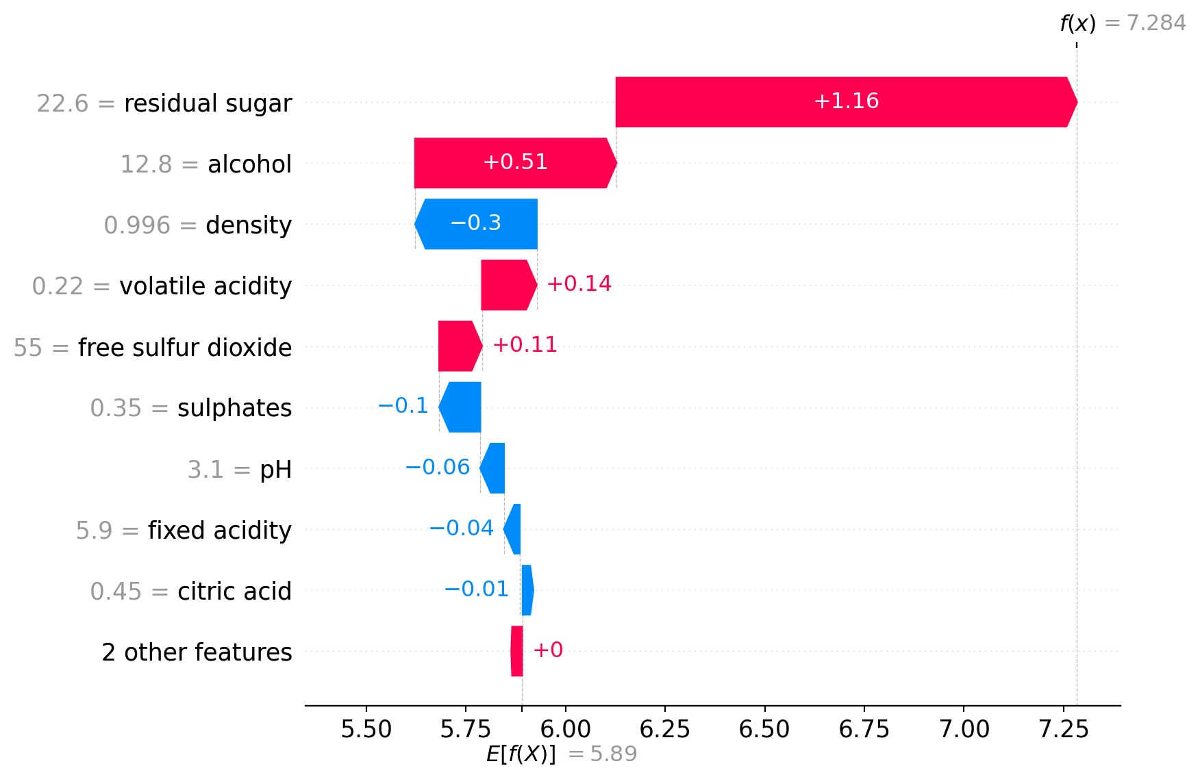
# Create SHAP explainer for linear models
explainer = shap.LinearExplainer(model, X_train)

# Compute SHAP values for test set
shap_values = explainer(X_test)

print(f"SHAP values shape: {shap_values.values.shape}")
print(f"Base value (average prediction): {shap_values.base_values[0]:.3f}")
print(f"\nSHAP values for first test instance:")
for feature, value in zip(X.columns, shap_values.values[0]):
    print(f"  {feature:25s}: {value:+.4f}")
print(f"\nPrediction for first instance: {model.predict(X_test.iloc[[0]])[0]:.3f}")
print(f"Sum: base_value + sum(shap_values) = {shap_values.base_values[0] + shap_values.values[0].sum():.3f}")

SHAP values shape: (980, 11)
Base value (average prediction): 5.890

SHAP values for first test instance:
  fixed acidity            : -0.0348
  volatile acidity         : +0.0031
  citric acid              : -0.0055
  residual sugar           : +0.3151
  chlorides                : -0.0001
  free sulfur dioxide      : +0.1074
  total sulfur dioxide     : -0.0023
  density                  : +0.0256
  pH                       : -0.0654
  sulphates                : +0.0529
  alcohol                  : +0.0855

Prediction for first instance: 6.372
Sum: base_value + sum(shap_values) = 6.372

We use SHAP’s LinearExplainer, which computes exact SHAP values efficiently for linear models. The explainer is initialized with the model and training data (to compute the base value). For each test instance, SHAP returns: (1) base_value: the average prediction across training data, (2) shap_values: the contribution of each feature to deviation from base_value. Notice that base_value + sum(shap_values) equals the model’s prediction - this is the additivity property. For linear models, SHAP values have a simple form: shap_i = coef_i × (x_i - mean(x_i)). This makes linear models perfect for understanding SHAP.

SHAP Waterfall Plot: Local Explanation

# Select an interesting wine (high quality prediction)
idx = np.argmax(model.predict(X_test))
print(f"Selected wine index: {idx}")
print(f"Predicted quality: {model.predict(X_test.iloc[[idx]])[0]:.2f}")
print(f"Actual quality: {y_test.iloc[idx]}")

# Create waterfall plot
shap.plots.waterfall(shap_values[idx])

Selected wine index: 14
Predicted quality: 7.28
Actual quality: 5

The waterfall plot shows how SHAP builds up from the base value (average prediction ~5.88) to the final prediction for a specific wine. Read from bottom to top: we start at E[f(X)], then each feature either pushes the prediction higher (red, right) or lower (blue, left). For this high-quality wine, alcohol content adds the most positive contribution, followed by density and volatile acidity. The sum of all contributions equals f(x) - E[f(X)]. This visualization answers: “Why did the model predict THIS value for THIS wine?” It’s perfect for explaining individual predictions to stakeholders.

SHAP Summary Plot: Global Feature Importance

# Create summary plot (beeswarm)
shap.plots.beeswarm(shap_values)

The summary plot (also called beeswarm plot) aggregates SHAP values across ALL test instances to show global patterns. The Y-axis shows features ranked by importance (vertical spread). The X-axis shows SHAP values (impact on prediction). Color indicates feature value (red = high, blue = low). Key insights: (1) Alcohol is most important - high values (red) consistently push predictions higher (right), (2) Volatile acidity is second most important - high values push predictions lower (left), (3) Density shows strong negative relationship when high. Compare this to feature importance from tree models - SHAP provides the same ranking but with directionality. This plot answers: “Which features matter most GLOBALLY across all wines?”

SHAP Dependence Plot: Feature Relationships

# Create dependence plot for alcohol
shap.plots.scatter(shap_values[:, 'alcohol'])

The dependence plot shows the relationship between feature value (X-axis) and SHAP value (Y-axis) for a specific feature. For alcohol, we see a clear LINEAR relationship - as alcohol increases, SHAP value increases proportionally. This makes perfect sense for a linear model! The color indicates interaction effects with another feature (automatically selected by SHAP). The vertical spread at each X value shows variance across instances. This plot answers: “HOW does this feature affect predictions?” For linear models, you’ll always see straight lines. For non-linear models (trees, neural networks), these plots reveal non-linear patterns, thresholds, and interactions.

Verifying SHAP Values for Linear Models

# For linear models: SHAP = coefficient × (x - mean(x))
# Let's verify this relationship

print("Verification: SHAP values = coefficient × (feature - mean)")
print("\nFor the first test instance:")
print(f"{'Feature':<25} {'Coefficient':>12} {'Value':>10} {'Mean':>10} {'(Val-Mean)':>12} {'SHAP Value':>12} {'Match?':>8}")
print("-" * 105)

for i, feature in enumerate(X.columns):
    coef = model.coef_[i]
    value = X_test.iloc[0][feature]
    mean = X_train[feature].mean()
    expected_shap = coef * (value - mean)
    actual_shap = shap_values.values[0][i]
    match = "✓" if np.isclose(expected_shap, actual_shap, rtol=1e-3) else "✗"
    print(f"{feature:<25} {coef:>12.4f} {value:>10.2f} {mean:>10.2f} {value-mean:>12.2f} {actual_shap:>12.4f} {match:>8}")

Verification: SHAP values = coefficient × (feature - mean)

For the first test instance:
Feature                    Coefficient      Value       Mean   (Val-Mean)   SHAP Value   Match?
---------------------------------------------------------------------------------------------------------
fixed acidity                   0.0459       6.00       6.87        -0.87      -0.0348        ✗
volatile acidity               -1.9149       0.29       0.28         0.01       0.0031        ✗
citric acid                    -0.0613       0.41       0.33         0.08      -0.0055        ✗
residual sugar                  0.0712      10.80       6.45         4.35       0.3151        ✗
chlorides                      -0.0265       0.05       0.05         0.00      -0.0001        ✗
free sulfur dioxide             0.0051      55.00      35.09        19.91       0.1074        ✗
total sulfur dioxide           -0.0002     149.00     138.00        11.00      -0.0023        ✗
density                      -124.2641       0.99       0.99        -0.00       0.0256        ✗
pH                              0.6007       3.09       3.19        -0.10      -0.0654        ✗
sulphates                       0.6491       0.59       0.49         0.10       0.0529        ✗
alcohol                         0.2290      10.97      10.51         0.46       0.0855        ✗

This verification slide demonstrates the elegant simplicity of SHAP for linear models. For each feature, SHAP value equals: coefficient × (feature_value - mean_feature_value). This shows that: (1) SHAP respects the linear model’s coefficients (direction and magnitude), (2) SHAP measures deviation from the mean (why predictions differ from average), (3) Features with large coefficients AND large deviations have high SHAP values. This is why linear models are perfect for teaching SHAP - you can directly see what SHAP computes. For non-linear models, SHAP still satisfies the same axioms, but the computation is more complex. The key insight: SHAP provides feature attributions that respect the model’s actual behavior.

Comparative Trade-offs: Choosing the Right XAI Tool

Criterion	PDP Partial Dependence Plot	LIME Local Interpretable Model-agnostic Explanations	SHAP SHapley Additive exPlanations
Scope	Global (feature-level)	Local (instance-level)	Both (local + global)
Primary Visualization	Line plot (2D curve)	Bar chart (sparse)	Force plot, Summary plot
Interpretability	★★★★★ Intuitive	★★★★☆ Easy to understand	★★★☆☆ Requires training
Computational Cost	★★★★☆ Moderate	★★★☆☆ Fast sampling	★★☆☆☆ Expensive
Theoretical Foundation	Statistical (marginal effects)	Heuristic (local approximation)	Game theory (Shapley values)
Feature Coverage	One at a time	Sparse (selected)	All features (dense)
Best For	Understanding global trends	Quick local explanations	Rigorous feature attribution
Key Limitation	Assumes independence	Unstable (sampling)	Computational cost

This table provides a decision guide for practitioners. Choose PDP when you need to understand how a feature affects predictions globally - great for presentations to stakeholders. Choose LIME when you need fast, interpretable explanations for individual predictions - ideal for production systems where speed matters. Choose SHAP when you need theoretically grounded attributions and can afford the computational cost - best for research or high-stakes decisions. In practice, use multiple methods: PDP for global insights, LIME for quick checks, SHAP for final validation. Remember: no method is perfect - always validate against domain knowledge and use visualizations to communicate effectively.