Deep Learning Visualization

CS-GY 9223 - Fall 2025

Claudio Silva

NYU Tandon School of Engineering

2025-10-27

Deep Learning Fundamentals

Agenda

Goal: Grasp foundational DL concepts essential for understanding network visualization techniques.

1. Deep Learning Terminology and Foundations

2. Linear Models and Loss Functions

3. Shallow Neural Networks and Activation Functions

4. Deep Neural Networks and Composition

5. Interactive Visualization Tools

Acknowledgments:

Materials adapted from:

• Prince, S. J. D. (2023). Understanding Deep Learning. MIT Press.

Today we transition from traditional ML interpretation methods to deep learning visualization. Deep learning models are the ultimate “black boxes” - millions of parameters organized in complex hierarchical structures. This lecture provides foundational understanding of how neural networks work, which is essential for understanding visualization techniques in future lectures. We’ll progress from simple linear regression through shallow networks to deep architectures, building intuition step by step. The Understanding Deep Learning book by Simon Prince provides excellent visualizations that make these concepts accessible. This is intentionally a lighter lecture focusing on fundamentals, as it sets up more advanced topics like CNN visualization, attention mechanisms, and activation analysis in later sessions.

Important emphasis: Understanding the forward and backward pass (which we cover in the fundamentals) is essential for comprehending the visualizations we’ll use to debug and interpret models. The forward pass shows how data flows through the network to make predictions, while the backward pass (backpropagation) shows how gradients flow back to update parameters. Both are critical for understanding visualization techniques like activation maximization, saliency maps, and gradient-based attribution methods that we’ll explore in later lectures.

Understanding Deep Learning

Understanding Deep Learning by Simon J.D. Prince

Published by MIT Press, 2023

Available free online: https://udlbook.github.io/udlbook

Why this book?

• Modern treatment (includes transformers, diffusion models)
• Excellent visual explanations
• Free and accessible
• Strong mathematical foundations with intuitive explanations

The exceptionally clear visual explanations in Prince’s book are why we use it as a primary resource for this course. All figures in today’s lecture are adapted from this source for consistency, specifically from Chapters 2-4 which cover supervised learning, shallow networks, and deep networks. This is an outstanding modern resource that covers everything from neural network basics to cutting-edge architectures like transformers and diffusion models. Unlike older deep learning texts, it includes recent developments while maintaining exceptional visual clarity. The book is freely available online, making it accessible to all students. Prince strikes a balance between mathematical rigor and intuitive explanation - he provides the equations but also explains the “why” behind them, which aligns perfectly with our visualization-focused approach.

Deep Learning Terminology

The Supervised Learning Framework:

\[y = f[x, \Phi]\]

Symbol	Meaning	Example
\(y\)	Prediction (model output)	House price: $450,000
\(x\)	Input (features)	Square footage: 2000 sq ft, Bedrooms: 3
\(\Phi\)	Model parameters (weights, biases)	Millions of numbers learned from data
\(f[\cdot]\)	Model function (architecture)	Neural network with multiple layers

Key Insight: Deep learning learns the parameters \(\Phi\) from training data pairs \(\{x_i, y_i\}\) to minimize prediction errors.

This slide establishes the fundamental notation we’ll use throughout. The prediction y is our model’s output. The input x contains all features describing the data point. The parameters Φ (phi) are what the model learns during training - in deep networks this could be millions or even billions of numbers. The function f defines the model architecture - how inputs flow through layers to produce outputs. We learn Φ by showing the model many examples {x_i, y_i} and adjusting parameters to minimize errors. The key distinction of deep learning is that the model learns hierarchical representations (feature extraction) automatically through minimizing error, rather than requiring hand-crafted features.

The Learning Process

Training Data:

Pairs of inputs and outputs: \(\{x_i, y_i\}\)

Loss Function:

Quantifies prediction accuracy: \(L[\Phi]\)

• Lower loss = better fit to training data
• Guides parameter updates during training

Goal:

Find parameters \(\Phi\) that minimize \(L[\Phi]\)

\[\Phi^* = \arg\min_{\Phi} L[\Phi]\]

Generalization:

Test on separate data not seen during training

The Challenge:

We don’t want to just memorize training data!

We want models that generalize to new, unseen examples.

→ This is why we split data into train/validation/test sets.

The learning process has three key components: (1) TRAINING DATA: pairs of inputs and corresponding correct outputs. For image classification, this would be images paired with labels. For regression, features paired with target values. (2) LOSS FUNCTION: a scalar value that measures how well our current parameters perform. Common losses: mean squared error for regression, cross-entropy for classification. The loss is computed by comparing predictions f[x,Φ] to true outputs y across all training examples. (3) OPTIMIZATION: This is the systematic process of adjusting Φ to reduce the Loss, typically using Gradient Descent (covered next) and Backpropagation, which finds the error gradient. The critical concept: we care about GENERALIZATION not just training performance. A model that memorizes training data but fails on new data is useless. This is why we evaluate on held-out test data and why techniques like dropout and regularization are important.

Linear Models: Building Intuition

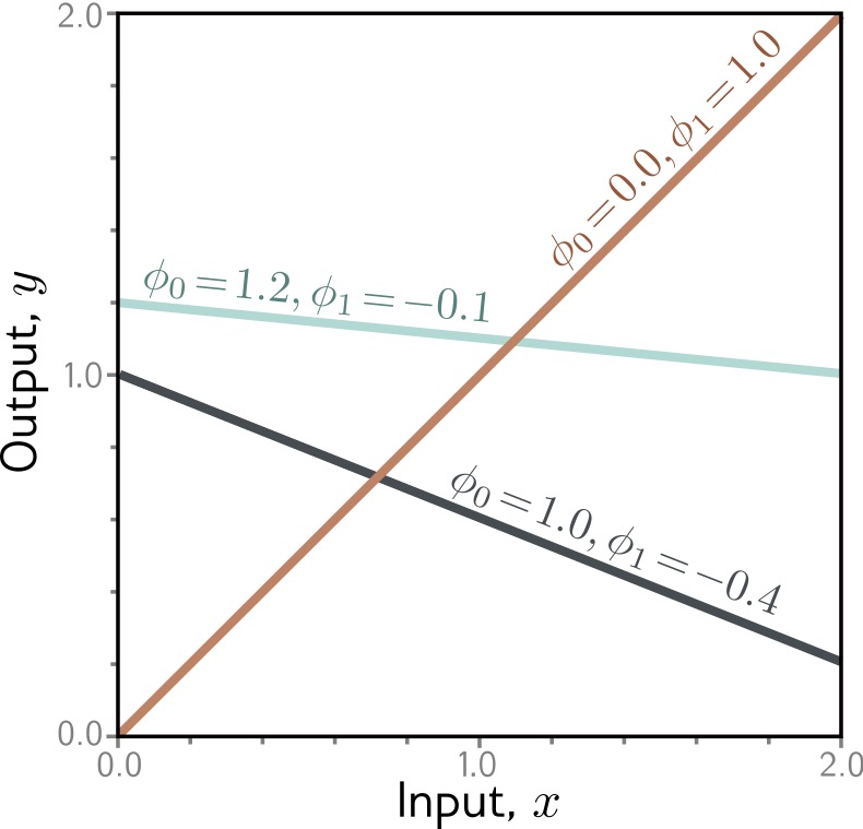
1-D Linear Regression Model

The simplest supervised learning model:

\[y = f[x, \Phi] = \Phi_0 + \Phi_1 x\]

• \(\Phi_0\): Intercept (bias term)
• \(\Phi_1\): Slope (weight)
• Only 2 parameters to learn

Let’s start with the absolute simplest case: linear regression in one dimension. We have one input feature x and one output y. The model has just two parameters: Φ₀ (intercept/bias) and Φ₁ (slope/weight). This is the familiar y = mx + b from algebra. The figure shows training data as dots and the fitted line. Even though this model is simple, it introduces all the key concepts: we have parameters to learn, we make predictions, and we can measure how good our predictions are. The limitations are obvious - many real-world relationships are non-linear. But understanding this simple case makes it easier to understand neural networks, which are essentially compositions of many non-linear transformations. Remind students this simple model is functionally equivalent to a single-neuron network with a linear activation function.

Linear Regression: Measuring Error

How do we quantify “good fit”?

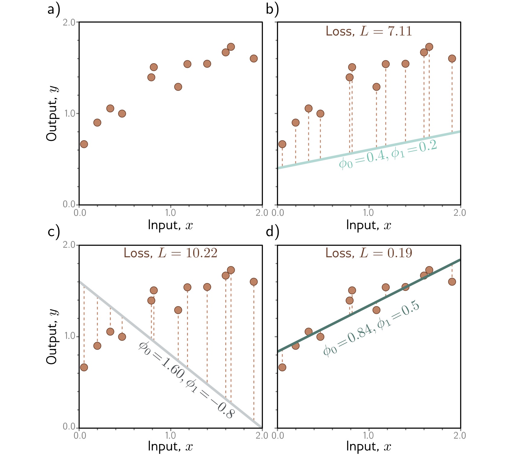
Loss Function: Sum of squared errors

\[L[\Phi] = \sum_{i=1}^{N} (y_i - f[x_i, \Phi])^2\]

Vertical distance from each data point to the line → squared → summed = total error

This visualization shows the concept of prediction error geometrically. For each training point (x_i, y_i), we compute the model’s prediction f[x_i, Φ]. The difference between true value y_i and prediction is the error (shown as vertical lines). We square these errors to make them all positive and penalize large errors more heavily. Summing across all training points gives the total loss. The goal of training is to adjust the line’s position and slope to minimize this total squared error. Why square the errors? (1) Makes all errors positive (otherwise errors could cancel), (2) Penalizes large errors more than small ones (quadratic penalty), (3) Makes the math work out nicely for optimization (differentiable). This is the classic Least Squares / Mean Squared Error (MSE) principle, which is the default loss function for all regression tasks in deep learning.

Loss Surface

Visualizing all possible parameter combinations:

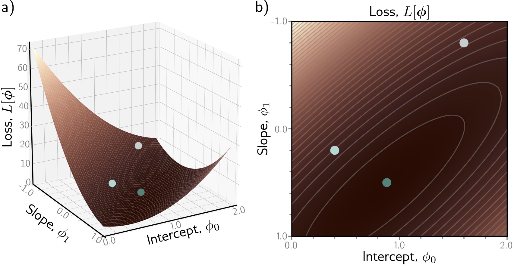
• X-axis: Slope \(\Phi_1\)
• Y-axis: Intercept \(\Phi_0\)
• Z-axis (color): Loss \(L[\Phi]\)

Goal: Find the lowest point (dark blue valley)

Key Observations:

1. Single global minimum - bowl-shaped surface
2. Smooth - we can use gradients to navigate
3. Convex - any path downhill leads to optimum

For linear models, optimization is easy! Deep networks have much more complex loss landscapes…

This is one of the most important visualizations for understanding optimization. Each point on this surface represents a different choice of parameters (Φ₀, Φ₁). The height/color represents the loss for those parameters. We start at some random point on this surface and want to reach the lowest point (minimum loss). For linear regression, this surface is convex (bowl-shaped) which makes optimization straightforward - just follow the gradient (steepest descent direction) and you’re guaranteed to reach the global minimum. Notice the smooth contours - this tells us the loss function is differentiable, which enables gradient-based optimization. IMPORTANT CONTRAST: Deep neural networks have extremely complex loss surfaces with many local minima, saddle points, and plateaus. The smooth bowl shape we see here is the exception not the rule. This is why training deep networks is challenging and requires careful techniques like adaptive learning rates, momentum, and batch normalization. Visualizing these complex deep learning loss landscapes—which are non-convex and have millions of dimensions—is a major topic later in the course. This contrast (convex vs. non-convex) is foundational.

Optimization: Gradient Descent

How do we find the minimum?

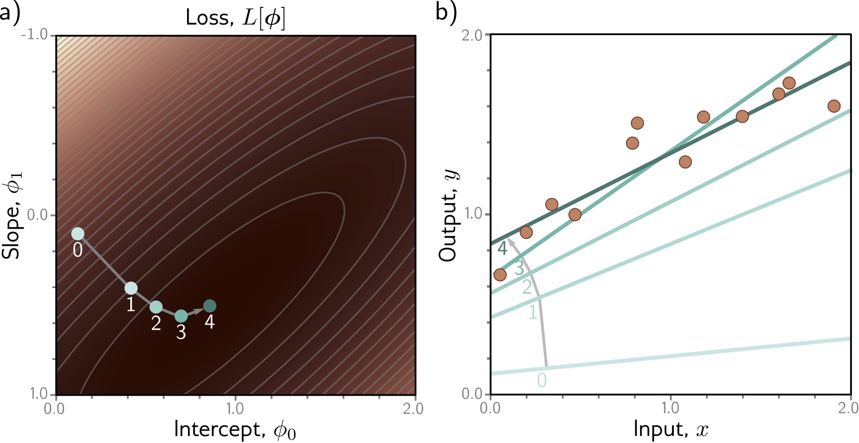
Algorithm: Iteratively move downhill

1. Start at random position
2. Compute gradient (slope direction)
3. Take small step opposite to gradient
4. Repeat until convergence

\[\Phi_{new} = \Phi_{old} - \alpha \nabla L[\Phi]\]

(\(\alpha\) = learning rate)

This visualization shows the optimization trajectory - the path taken through parameter space to reach the minimum. We start at a random initialization (usually small random values) and compute the gradient of the loss with respect to parameters. The gradient points in the direction of steepest ASCENT, so we move in the OPPOSITE direction to descend. The learning rate α controls step size. The figure shows several iterations converging to the optimal parameters (center of the bowl). KEY HYPERPARAMETER: Learning rate. Too large → overshoot and diverge. Too small → very slow convergence. For deep learning we use sophisticated optimizers (Adam, RMSprop) that adaptively adjust learning rates. The algorithm shown is Gradient Descent. To use it in a neural network, we need the Backpropagation algorithm to efficiently compute the gradient (∇L[Φ]) for all parameters using the chain rule. Gradient Descent is the steering, Backpropagation is the engine.

Shallow Neural Networks

From Linear to Non-linear

Linear models are limited - they can only learn straight lines!

Solution: Add non-linearity through activation functions

Transform linear combinations with a non-linear function → enables learning complex patterns

Shallow Neural Network (1 hidden layer):

\[y = f[x, \Phi] = \Phi_0 + \sum_{i=1}^{3} \Phi_i \cdot a[ \Theta_{i0} + \Theta_{i1} x]\]

Component	Description	Count
\(\Theta_{ij}\)	First layer parameters	6 parameters
\(\Phi_i\)	Second layer parameters	4 parameters
\(a[\cdot]\)	Activation function	Non-linearity!

Total: 10 parameters (vs 2 for linear model)

This is the critical leap from linear models to neural networks. A linear model can only learn linear relationships - straight lines in 1D, planes in higher dimensions. Real-world data often has non-linear patterns. The solution: compose multiple linear transformations with non-linear activation functions between them. The equation shows a shallow network with 3 hidden units. The input x is first transformed by 3 linear functions (with parameters Θ), then passed through activation function a[·], then linearly combined (with parameters Φ) to produce output y. We’ve gone from 2 parameters to 10 parameters, giving much more expressive power. The activation function is crucial - without it, composing linear transformations would just give another linear transformation. The non-linearity is what enables neural networks to approximate arbitrary functions. The network learns to combine these simple non-linear ‘basis functions’ (the hidden units) to approximate extremely complex mappings. This compositionality is the core power of NNs.

Activation Functions: ReLU

ReLU (Rectified Linear Unit): The most popular activation function

\[a[z] = \max(0, z) = \begin{cases} z & \text{if } z > 0 \\ 0 & \text{if } z \leq 0 \end{cases}\]

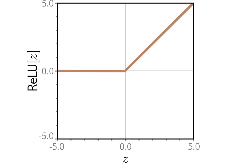
Why ReLU?

✓ Simple: Easy to compute and differentiate

✓ Efficient: Avoids vanishing gradient problem

✓ Sparse: Many activations are exactly zero

✓ Biological: Neurons either fire or they don’t

ReLU is the workhorse activation function of modern deep learning. It’s incredibly simple: output the input if positive, otherwise output zero. This creates a “bent” linear function - linear for positive inputs, flat for negative. The figure shows how ReLU transforms various inputs. Why is this simple function so powerful? (1) COMPUTATIONAL EFFICIENCY: Just a comparison and max operation, much faster than sigmoid or tanh which require exponentials. (2) GRADIENT FLOW: For positive inputs, gradient is 1, which helps avoid the vanishing gradient problem that plagued older networks. (3) SPARSITY: Roughly half of activations are exactly zero, which can improve generalization and efficiency. (4) BIOLOGICAL PLAUSIBILITY: Resembles neuron behavior - neurons have a threshold below which they don’t fire. A common issue is the ‘Dying ReLU’ problem (when z ≤ 0, the gradient is 0, halting learning for that neuron). Variants like Leaky ReLU address this by giving a small slope to negative values. Other variants include Parametric ReLU and GELU, but standard ReLU remains the most common. The simplicity is a feature not a bug - it works remarkably well in practice.

Building Intuition: Composing ReLUs

How do multiple ReLU activations combine to approximate complex functions?

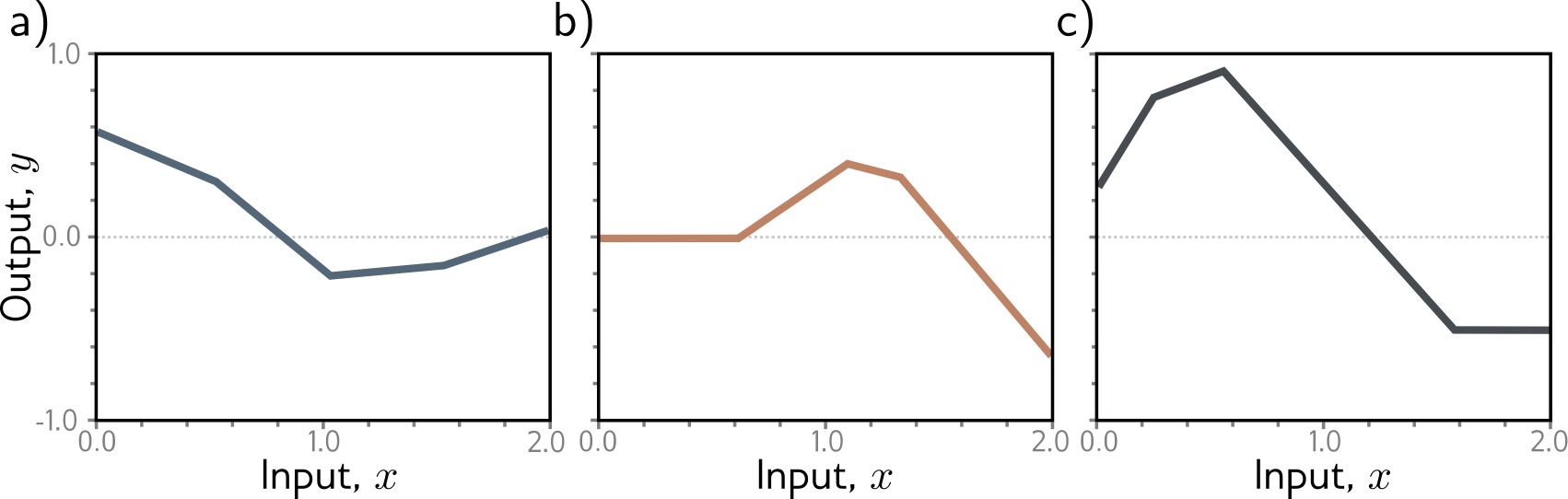
Each hidden unit:

1. Computes linear function of input
2. Applies ReLU → bent line
3. Gets weighted and summed

Combining multiple units:

• Different slopes and bends
• Sum creates complex shapes
• More units → more flexibility

This visualization shows how individual ReLU units (bent lines) combine to approximate a more complex function. Each row shows a different hidden unit’s contribution: (1) a linear transformation of the input, (2) ReLU applied (creating the bend), (3) weighted by the second-layer parameter Φ. The bottom row shows the sum of all these bent lines, which can approximate surprisingly complex shapes. Think of each hidden unit as creating a “hinge” in the function at a different location and with a different angle. By combining multiple hinges, we can approximate nearly any continuous function. The more hidden units, the more hinges, the more complex the function we can represent. This builds intuition for why neural networks are such powerful function approximators.

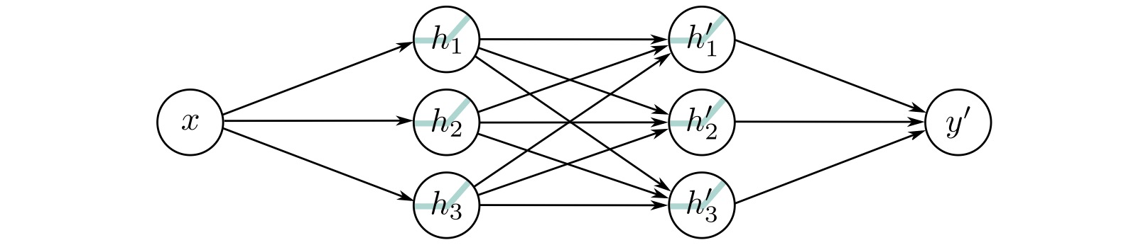
Neural Network Computation

Step-by-step: How a shallow network processes an input

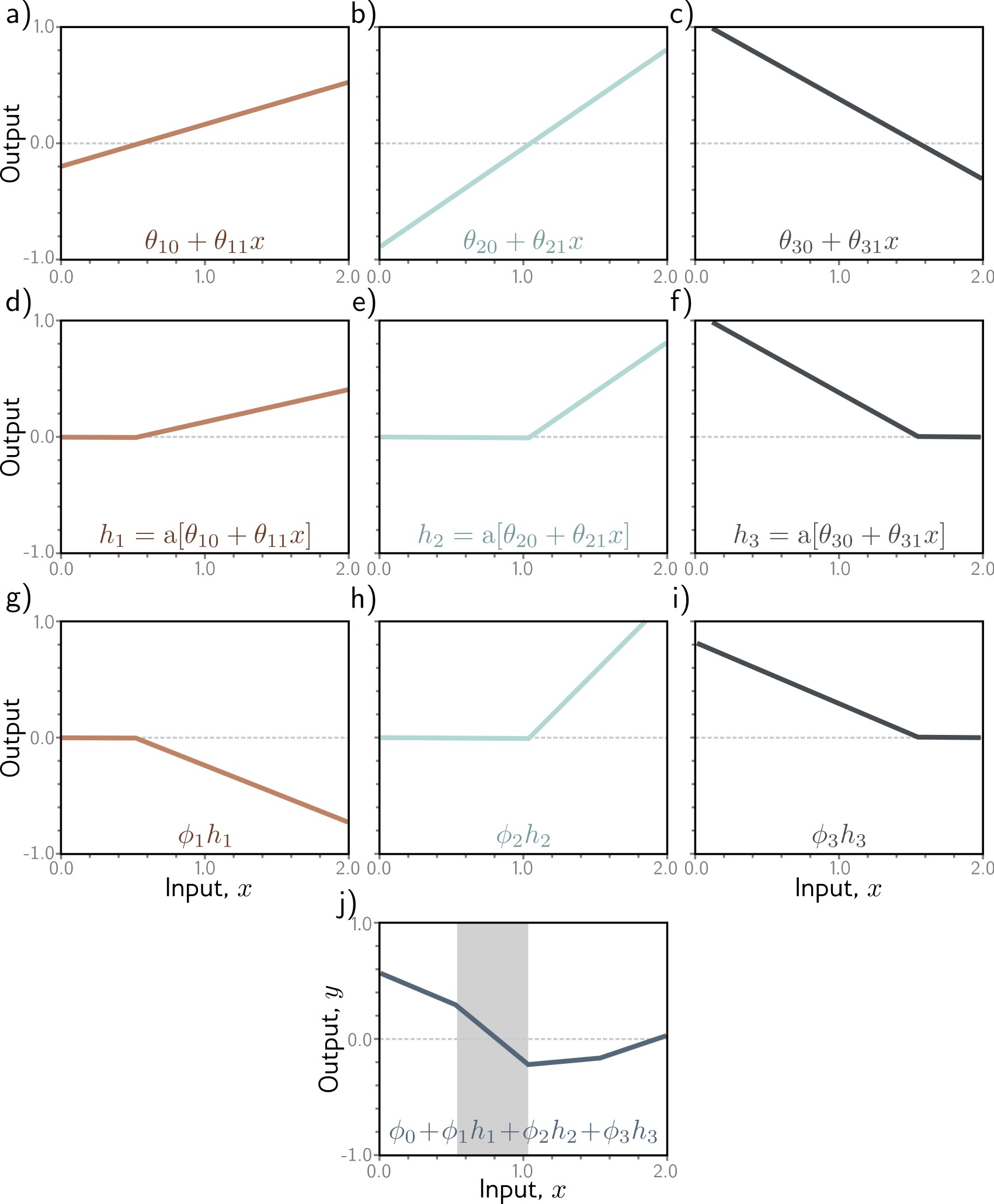
Process:

1. Input \(x\) (left) enters the network

2. Each hidden unit computes: \(h_i = a[\Theta_{i0} + \Theta_{i1} x]\)

3. Weighted combination: \(y = \Phi_0 + \sum_i \Phi_i h_i\)

4. Final output \(y\) (right)

This slide shows the Forward Pass (prediction). This sequential visualization shows how information flows forward through a shallow network. We start with input x on the left. This input is sent to each of 3 hidden units in parallel. Each hidden unit computes a weighted sum (linear transformation) and applies ReLU. These hidden activations are then weighted and summed to produce the final output y. This is called “forward propagation” - information flows forward from input to output to compute the prediction. Remember that training requires the Backward Pass (Backpropagation), which computes the gradients by applying the chain rule backwards from the loss to the input layer. The figure helps visualize the layer structure: input layer (just the raw features), hidden layer (computed representations), output layer (final prediction). Modern deep networks have many hidden layers, but the principle is the same.

Neural Network Diagram

Standard visualization: Network architecture

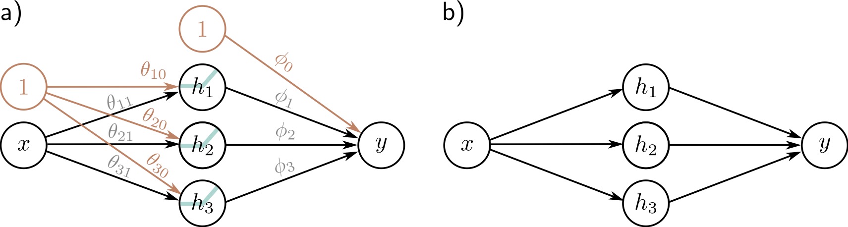
Components:

• ⚫ Input layer: Raw features
• 🔵 Hidden layer: Learned representations
• ⚫ Output layer: Prediction
• → Connections: Weighted parameters

Terminology:

• Hidden units/neurons: Computed values in middle
• Pre-activations: Before ReLU
• Activations: After ReLU
• Fully connected: Every unit connects to all units in next layer

This is the classic neural network diagram you see everywhere. Each circle represents a unit (neuron), lines represent weighted connections (parameters). Information flows left to right during forward propagation. LAYER TERMINOLOGY: (1) INPUT LAYER: Not really a “layer” - just the input features. No computation happens here. (2) HIDDEN LAYER: Called “hidden” because these values are internal to the model, not directly observable. The hidden layer is where the network learns an entirely new intermediate representation of the input data that is more useful for the final task. This is why we call it feature learning. (3) OUTPUT LAYER: Final prediction. For regression this is one unit, for multi-class classification it’s one unit per class. FULLY CONNECTED: Each unit connects to all units in the next layer. This is also called “dense” layer. Modern architectures (CNNs, Transformers) use different connectivity patterns, but fully-connected is the building block. The term “shallow” means just one hidden layer. “Deep” means multiple hidden layers stacked.

Universal Approximation Theorem

Theoretical Foundation: Shallow networks can approximate any continuous function!

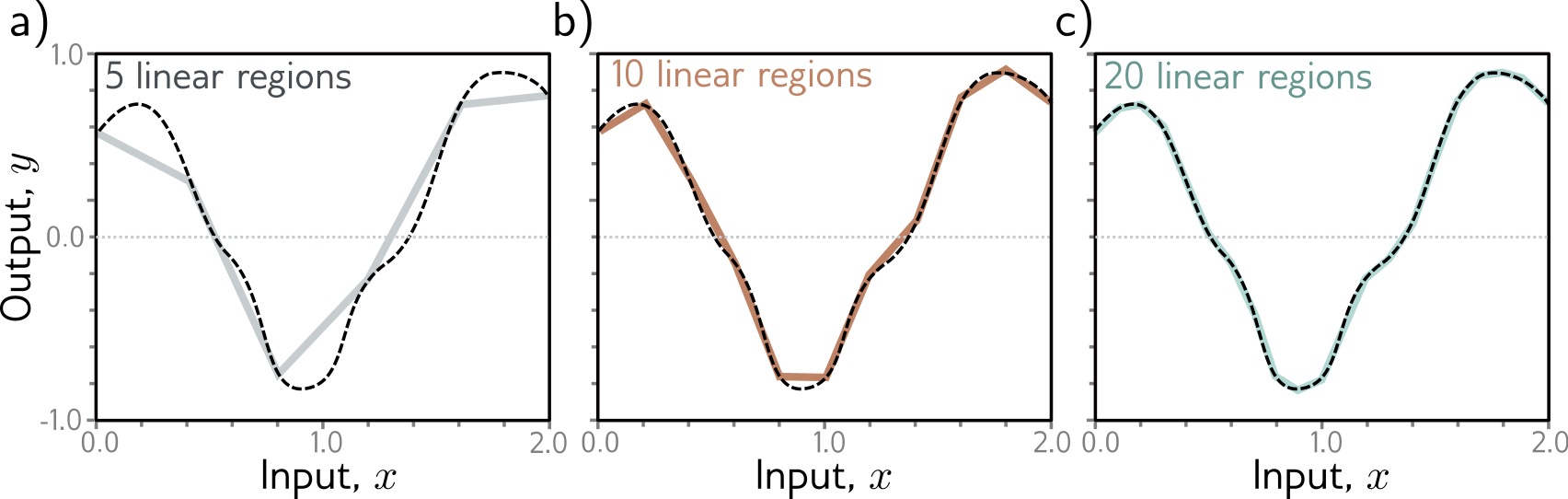
Theorem (Cybenko 1989, Hornik 1991):

A shallow neural network with enough hidden units can approximate any continuous function to arbitrary accuracy on a compact domain.

But…

• May require exponentially many hidden units
• Doesn’t tell us how to find the parameters
• Deep networks are often more efficient

The Universal Approximation Theorem is a profound theoretical result. It says that given enough hidden units, a shallow network (just one hidden layer) can approximate any continuous function you can draw. The figure illustrates this - as we add more hidden units, the approximation gets better and better. This is why neural networks are so powerful! HOWEVER, there are crucial caveats: (1) “Enough hidden units” might mean exponentially many as the input dimension grows. For complex functions in high dimensions, a shallow network might need billions of units. (2) The theorem says such a network EXISTS but doesn’t tell us how to find the right parameters through training. (3) Even if we could find the parameters, the network might generalize poorly. The key takeaway is that a shallow network is theoretically enough, but practically inefficient for large, high-dimensional problems. We use depth to achieve the same approximation power with far fewer total parameters. Deep networks exploit compositionality and hierarchy. Think of it like computer code: you COULD write any program as one giant function, but it’s much more efficient to compose smaller functions.

Deep Neural Networks

Why Go Deep?

Deep networks compose simple transformations to build complex representations

Shallow network limitations:

• Requires many hidden units
• Doesn’t exploit structure
• Inefficient representation

Deep network advantages:

• Hierarchical learning
• Compositional structure
• Parameter efficiency
• Feature reuse across layers

Intuition from vision:

Layer 1: Edges, colors

↓

Layer 2: Textures, simple shapes

↓

Layer 3: Object parts

↓

Layer 4: Object categories

Each layer builds on previous representations!

This slide motivates why deep architectures are so powerful. Shallow networks can theoretically approximate any function, but deep networks do it much more efficiently by exploiting compositional structure. Think about how humans understand images: we don’t process pixels directly into “cat” or “dog”. We first detect edges, then combine edges into textures, textures into parts (ears, nose), parts into objects. This is HIERARCHICAL composition - each level builds on the previous. Deep networks learn similar hierarchies automatically! Early layers learn simple features (edges in images, syllables in audio), middle layers combine them into parts (object parts, words), late layers capture high-level concepts (object categories, sentence meaning). This compositionality gives exponential representational power - k layers with n units per layer can represent exponentially more functions than kn units in a single layer. This is similar to how compound words work - “black”, “board” → “blackboard” has new meaning beyond the parts.

Composing Networks

Building deep networks: Stack multiple hidden layers

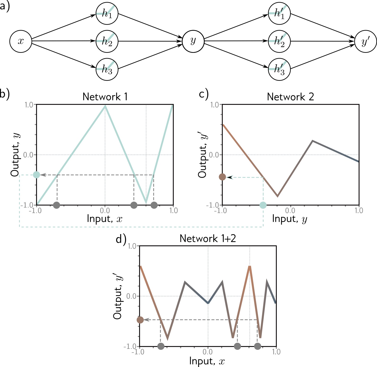
Each layer:

\[h^{(k)} = a[W^{(k)} h^{(k-1)} + b^{(k)}]\]

• \(h^{(k)}\): Activations at layer \(k\)

• \(W^{(k)}\), \(b^{(k)}\): Parameters for layer \(k\)

• Composition: \(f = f_K \circ f_{K-1} \circ \ldots \circ f_1\)

This visualization shows how we build deep networks by composing multiple layers. Each layer performs the same operation: linear transformation (W*h + b) followed by non-linearity (activation function a). The output of layer k becomes the input to layer k+1. The overall function is a composition f = f_K ∘ f_{K-1} ∘ … ∘ f_1, where each f_k represents one layer. The notation h^(k) represents the hidden activations at layer k - these are the learned representations at that depth. Early layers (close to input) learn low-level features, later layers (close to output) learn high-level concepts. This composition is what gives deep learning its power. During backpropagation, gradients flow backwards through this composition using the chain rule - this is how we learn parameters for all layers simultaneously.

How Deep Networks Transform Space

Geometric intuition: Each layer performs a non-linear transformation of the representation space

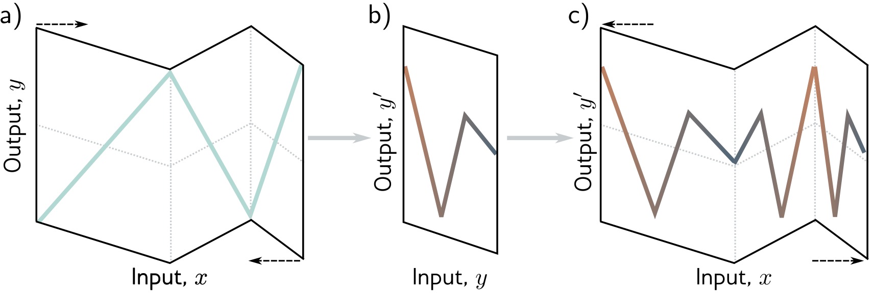
Layer 1:

Stretches, rotates, bends space with ReLU

Layer 2:

Further transforms the already-bent space

Result:

Complex folding of input space

→ Can separate classes that were originally intertwined

This is a beautiful geometric visualization of what deep networks do. Think of the input space as a rubber sheet. Each layer applies a transformation that stretches, compresses, rotates, and folds this sheet. ReLU creates sharp bends (folding). Linear transformations create stretching and rotation. The figure shows how two classes (two different colors) that might be intertwined in the original input space get separated into distinct regions after the transformations. This is why deep networks can solve complex classification problems - they learn to warp the input space in ways that make classes linearly separable in the final layer. This geometric view helps understand: (1) Why depth matters - more folding operations can handle more complex decision boundaries. (2) Why ReLU matters - piecewise linear functions create the folds. (3) How representations change - each layer creates a new geometric space with different properties.

Two Hidden Layers

Adding depth: 2 hidden layers → more complex functions

Key difference from shallow networks:

• First layer creates intermediate representations
• Second layer operates on those representations, not raw inputs
• Can capture compositional structure

Example: First layer detects edges, second layer combines edges into shapes

This shows the architecture of a network with two hidden layers. The key insight: the second hidden layer doesn’t see the raw input - it sees the TRANSFORMED representations from the first hidden layer. This enables hierarchical feature learning. Each layer builds on the features learned by previous layers. With just two layers, we’re already seeing significant gains in representational power. The first layer might learn to detect simple patterns (edges, corners in images; phonemes in audio; word presence in text). The second layer combines these simple patterns into more complex ones (object parts; words; sentence structure). This composition is much more powerful and parameter-efficient than having one huge hidden layer. Modern deep networks typically have dozens or hundreds of layers, each learning progressively more abstract representations.

K Hidden Layers: Deep Architecture

Modern deep learning: Many layers stacked together

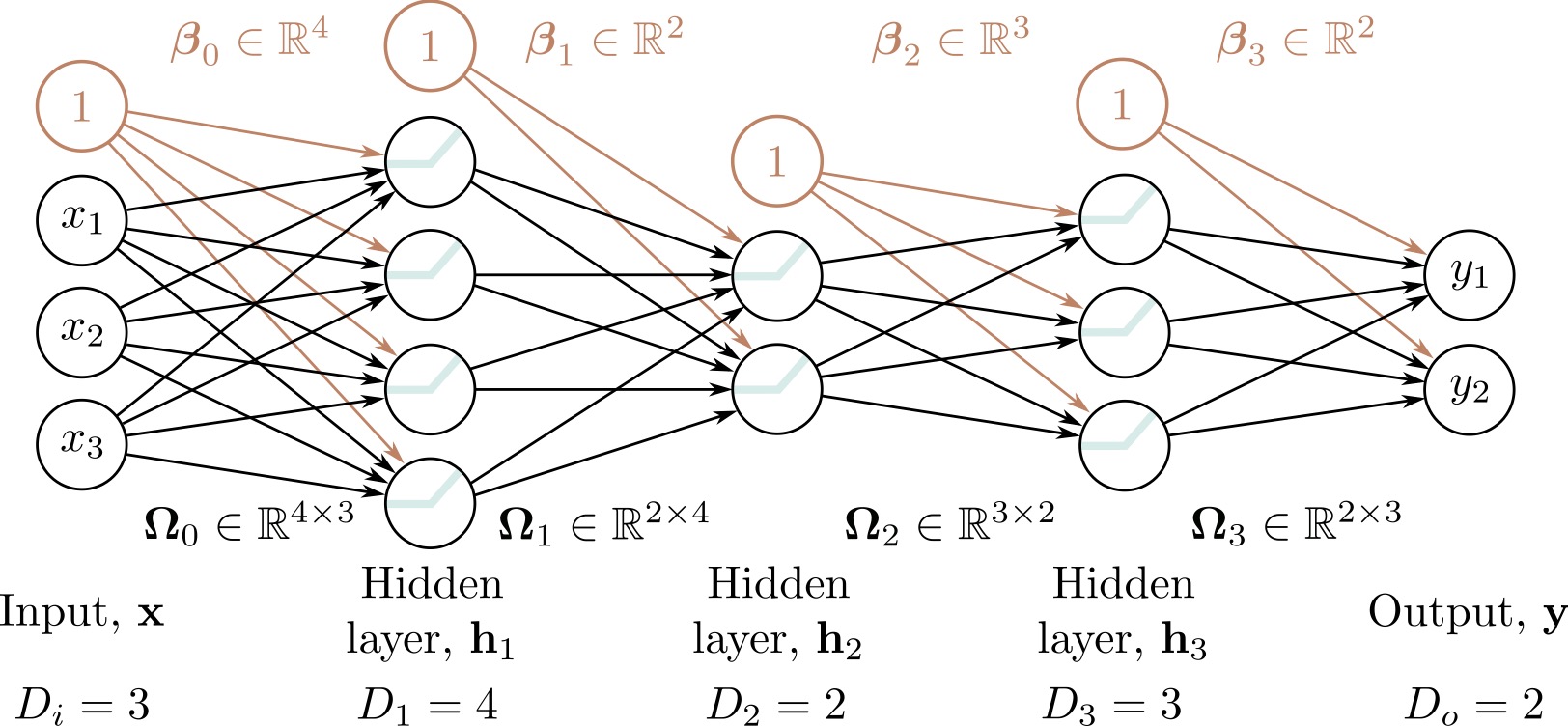
Deep Network Characteristics:

• Input layer: Raw features (e.g., pixel values)
• Hidden layer 1: Low-level features (edges, textures)
• Hidden layer 2: Mid-level features (parts, patterns)
• Hidden layer K: High-level features (concepts, objects)
• Output layer: Final prediction

Modern architectures: ResNet (152 layers), GPT-3 (96 layers), Vision Transformers (24+ layers)

Depth is power, but it comes with challenges like vanishing gradients and degradation. The solutions (like Residual Connections and Batch Normalization) are what enable modern deep learning to scale. This diagram shows a fully deep architecture with K hidden layers. Modern deep networks typically have many layers - ResNets for computer vision use 50-152 layers, transformer models like GPT-3 use 96 layers, and some experimental architectures exceed 1000 layers! Each additional layer allows the network to learn more abstract and compositional features. However, simply stacking layers creates challenges: (1) VANISHING GRADIENTS: Gradients become exponentially small as they backpropagate through many layers, making early layers hard to train. (2) DEGRADATION: Very deep networks can perform worse than shallower ones if not designed carefully. Modern architectures address these with techniques like: Residual connections (ResNet) that create shortcuts for gradient flow, Batch normalization that stabilizes activations, Careful initialization schemes, Adaptive optimizers like Adam. The visualization helps understand the information flow: data enters at the bottom/left, gets progressively transformed, and emerges as a prediction at the top/right.

Interactive Visualization Tools

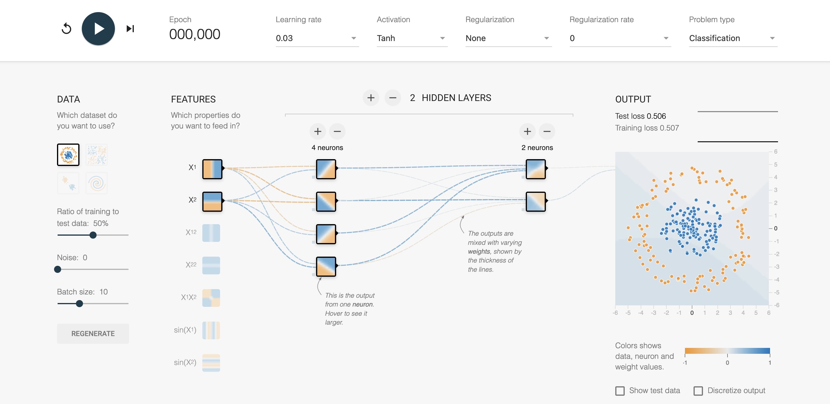
TensorFlow Playground

Interactive tool for understanding neural networks

https://playground.tensorflow.org

TensorFlow Playground is an outstanding interactive visualization for building intuition about neural networks. You can: (1) Choose different 2D datasets (spirals, circles, XOR, etc.) and see how networks learn decision boundaries. (2) Add/remove hidden layers and neurons to see how architecture affects learning. (3) Adjust learning rate and activation functions. (4) Watch training in real-time - see how decision boundaries evolve. (5) Observe individual neuron activations and how they combine. KEY INSIGHTS students gain: (1) Seeing how adding layers helps with complex patterns - try the spiral dataset with 1 vs 2 vs 4 hidden layers. (2) Understanding overfitting - watch what happens with too many neurons. (3) Observing feature learning - each neuron learns to detect a particular pattern. (4) Experiencing the effect of learning rate - too high causes oscillation, too low is very slow. Highly recommend students try to solve the Spiral Dataset with a single hidden layer, and then observe how easily it is solved when you add a second layer. It’s the best visual proof of why depth matters.

CNN Explainer

Interactive visualization for understanding Convolutional Neural Networks

https://poloclub.github.io/cnn-explainer/

CNN Explainer is a brilliant interactive tool from Georgia Tech that visualizes how convolutional neural networks process images. It shows: (1) LAYER-BY-LAYER visualization: See exactly how feature maps are computed at each layer. (2) FILTER VISUALIZATION: Examine what patterns individual convolutional filters detect. (3) ACTIVATION MAPS: Observe which parts of the image activate each neuron. (4) ARCHITECTURE OVERVIEW: Understand how conv layers, pooling, and fully-connected layers connect. (5) INTERACTIVE EXPLORATION: Click on neurons to trace their computation. This tool visually confirms the hierarchical feature learning we discussed: you can click on neurons to see exactly how early filters detect simple lines and how later filters combine those into complex object parts. This is particularly valuable because CNNs are the dominant architecture for computer vision, and understanding convolution operations is crucial. Students can: Upload their own images and watch them propagate through the network. See why early layers detect edges and later layers detect complex objects. Understand pooling (spatial downsampling) and how it provides translation invariance. We’ll cover CNNs in more detail in a future lecture on deep learning visualization, but this tool is excellent for building initial intuition.

Further Exploration

Recommended interactive visualizations and resources:

Neural Network Visualization:

• Distill.pub: The Building Blocks of Interpretability Comprehensive visual explanations

• TensorFlow Embedding Projector Explore high-dimensional embeddings

• ML4A: Looking Inside Neural Nets Interactive tutorials and visualizations

Understanding Deep Learning:

📖 udlbook.github.io/udlbook

Free online textbook with: - Interactive Python notebooks - Video lectures - Extensive visualizations - Modern coverage (transformers, diffusion models)

These resources provide excellent ways to deepen understanding beyond this lecture. DISTILL.PUB has become the gold standard for visual explanations of ML concepts - their articles on neural network interpretability are outstanding, combining interactive visualizations with rigorous explanations. The TensorFlow Embedding Projector lets you explore high-dimensional data (like word embeddings) using dimensionality reduction techniques like PCA and t-SNE. ML4A (Machine Learning for Artists) provides accessible tutorials with beautiful interactive visualizations. The Understanding Deep Learning book website has companion materials including Python notebooks that implement everything from scratch, making it perfect for hands-on learning. ENCOURAGE STUDENTS to explore these interactively. Reading about neural networks is good, but SEEING and MANIPULATING visualizations builds much deeper intuition. Spend 30 minutes playing with TensorFlow Playground and you’ll understand neural networks better than reading 100 pages of equations.

Summary: Deep Learning Foundations

Key Takeaways:

1. Supervised Learning: Learn parameters \(\Phi\) from data pairs \(\{x_i, y_i\}\) to minimize loss \(L[\Phi]\)

2. From Linear to Non-linear: Activation functions (ReLU) enable learning complex patterns

3. Shallow Networks: Single hidden layer can approximate any function (Universal Approximation Theorem)

4. Deep Networks: Multiple layers learn hierarchical representations more efficiently

5. Geometric View: Networks transform input space through non-linear folding to separate classes

Next lectures: We’ll explore specialized visualizations for CNNs, attention mechanisms, activation analysis, and network interpretability

Let’s consolidate what we’ve learned. We started with the basic supervised learning setup - learning a function that maps inputs to outputs by minimizing a loss function. We saw how linear models are limited and how adding non-linear activation functions (especially ReLU) enables neural networks to approximate complex functions. The Universal Approximation Theorem gives theoretical justification - shallow networks have tremendous representational power. However, deep networks are more practical because they exploit compositional structure and learn hierarchical representations efficiently. We developed geometric intuition: networks progressively transform the input space through non-linear warping, separating classes that were originally intertwined. LOOKING AHEAD: This lecture established foundations. In future lectures we’ll dive deeper into visualization techniques specific to different architectures: How to visualize what CNN filters detect, How attention mechanisms work in transformers, Techniques for activation maximization and feature visualization, Methods for network interpretability and debugging. The interactive tools (TensorFlow Playground, CNN Explainer) are excellent for building continued intuition.

Next Week: Topological Data Analysis

Preview of upcoming topic:

Topology meets machine learning

• Persistence diagrams and barcodes
• Mapper algorithm for visualization
• Reeb graphs
• Applications in ML and deep learning

Why it matters:

Topological Data Analysis (TDA) provides robust methods for understanding the shape and structure of high-dimensional data.

Essential for analyzing neural network representations, clustering, and feature spaces!

Next week we’ll explore Topological Data Analysis (TDA) - a powerful mathematical framework for understanding the shape and structure of complex, high-dimensional data. TDA provides tools that are robust to noise and capture global geometric properties that traditional methods miss. We’ll cover: Persistence diagrams and barcodes that summarize topological features across scales, The Mapper algorithm for creating insightful visualizations of high-dimensional datasets, Reeb graphs for understanding data topology, Applications to neural network analysis and representation learning. TDA is particularly valuable for ML because: It reveals clustering structure without choosing the number of clusters, It identifies loops, voids, and connected components in data, It’s robust to noise and outliers, It connects naturally to deep learning representations. The combination of today’s deep learning foundations plus next week’s TDA will give you powerful tools for understanding what complex models learn.