Clustering and Dimensionality Reduction
CS-GY 6313 - Fall 2026 - Instructor: Claudio Silva
2026-11-13
Clustering
Etienne Bernard: “… the goal of clustering is to separate a set of examples into groups called clusters”
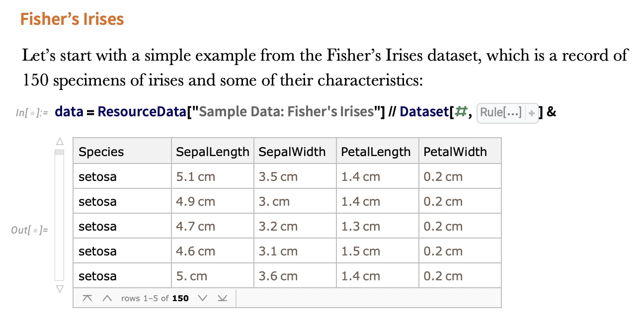
IRIS – another look
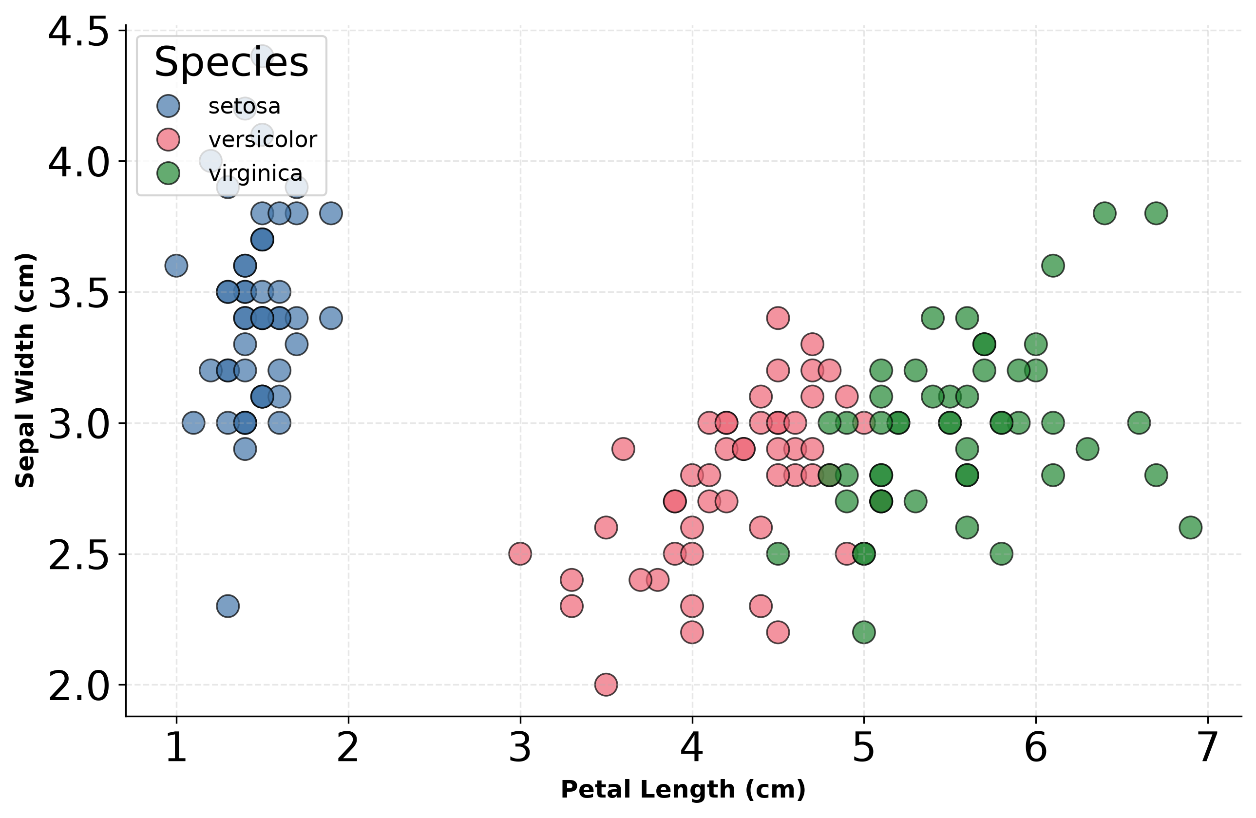
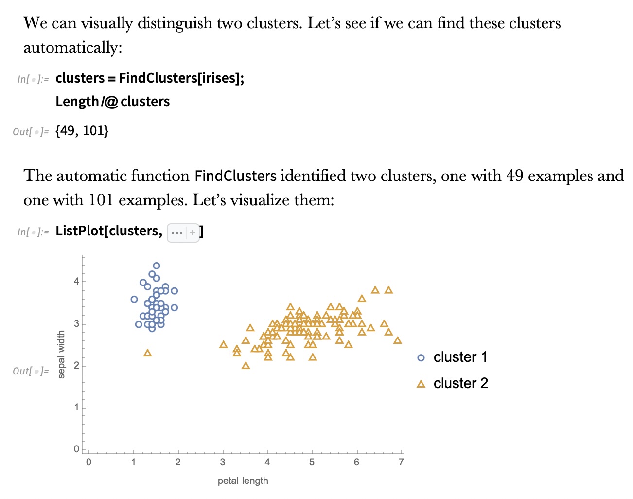
IRIS – clustering
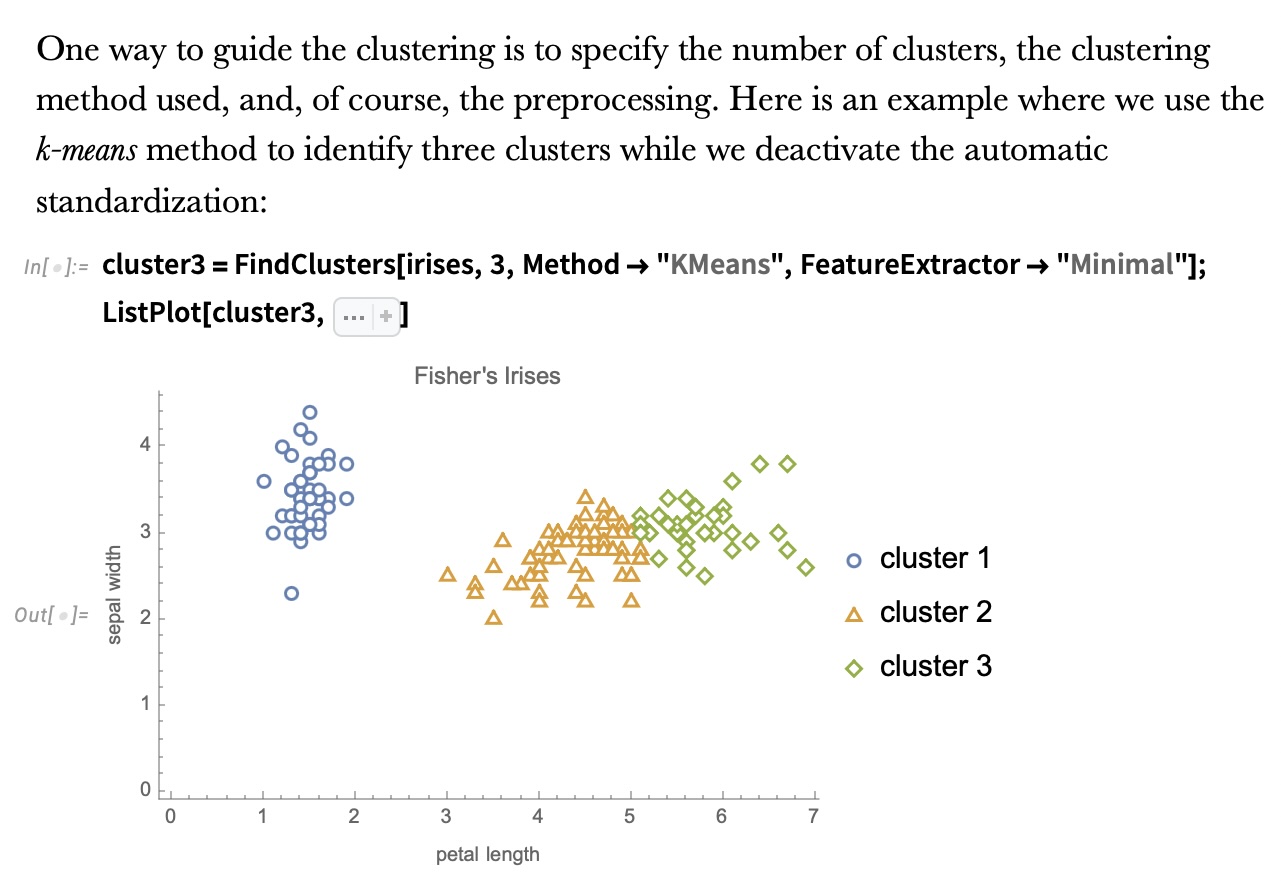
IRIS – k-means
Wolfram Mathematica FindClusters
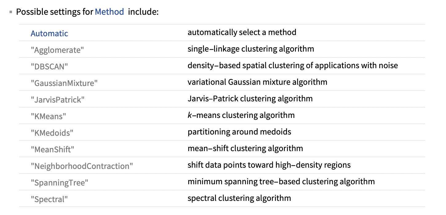
Wolfram Mathematica FindClusters
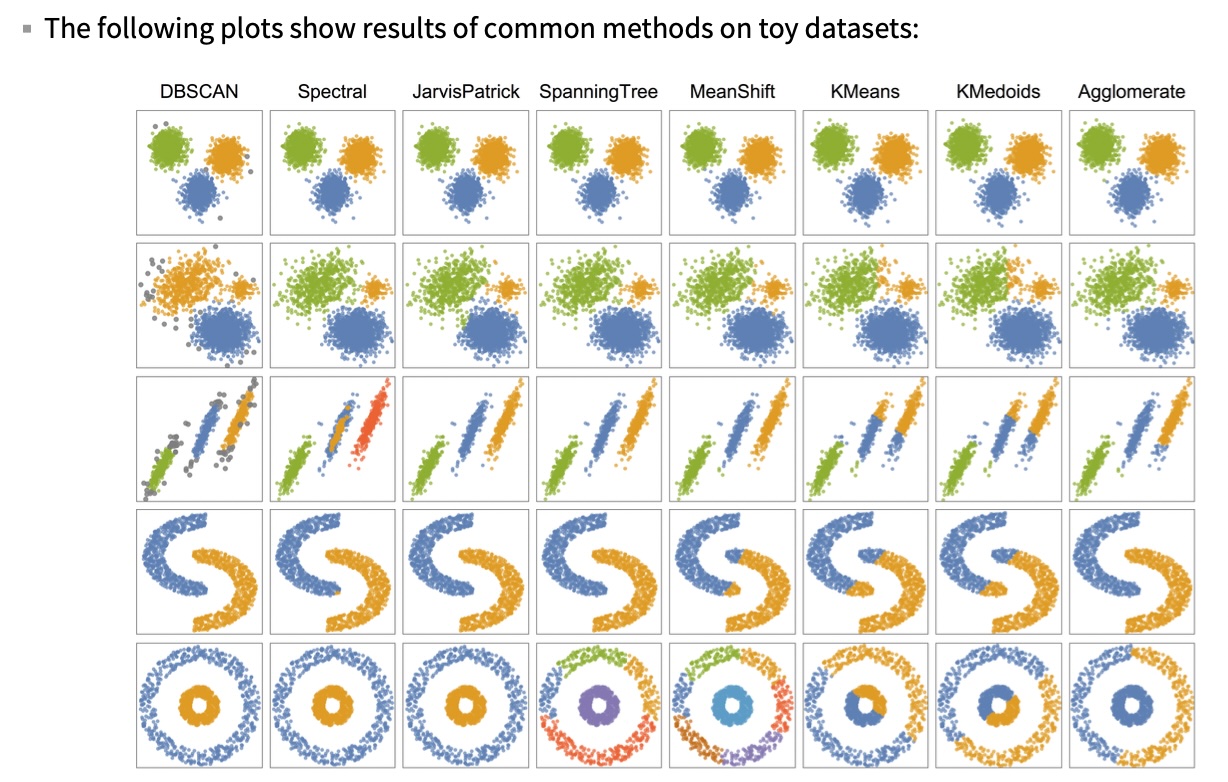
When k-means fails: shape, not count
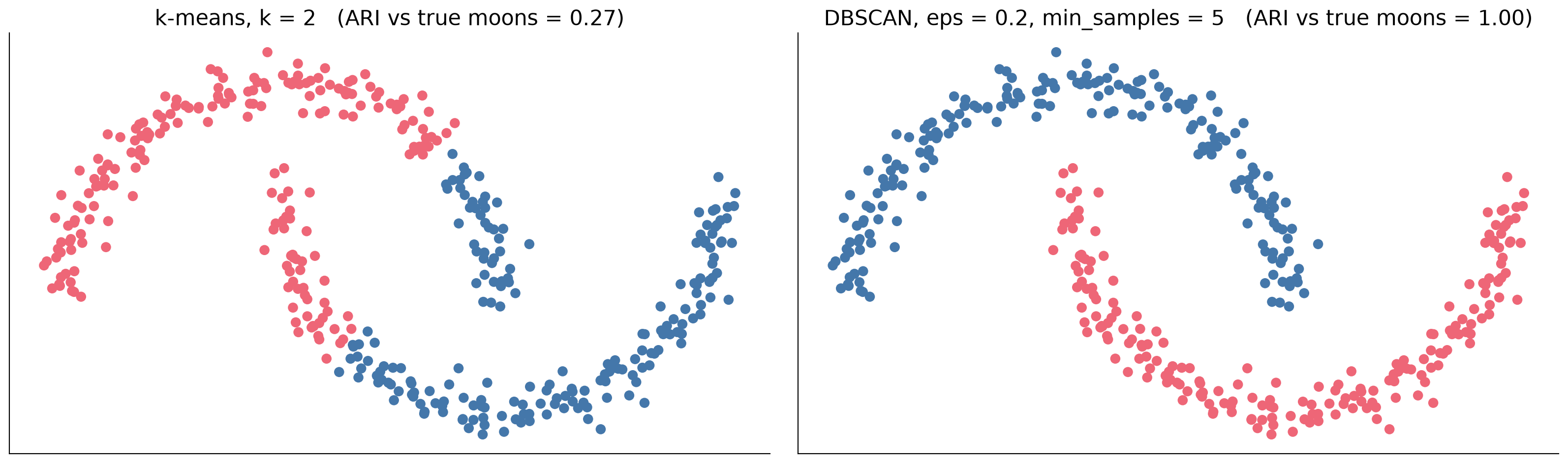
Right number of clusters, wrong definition of a cluster.
IRIS - classes
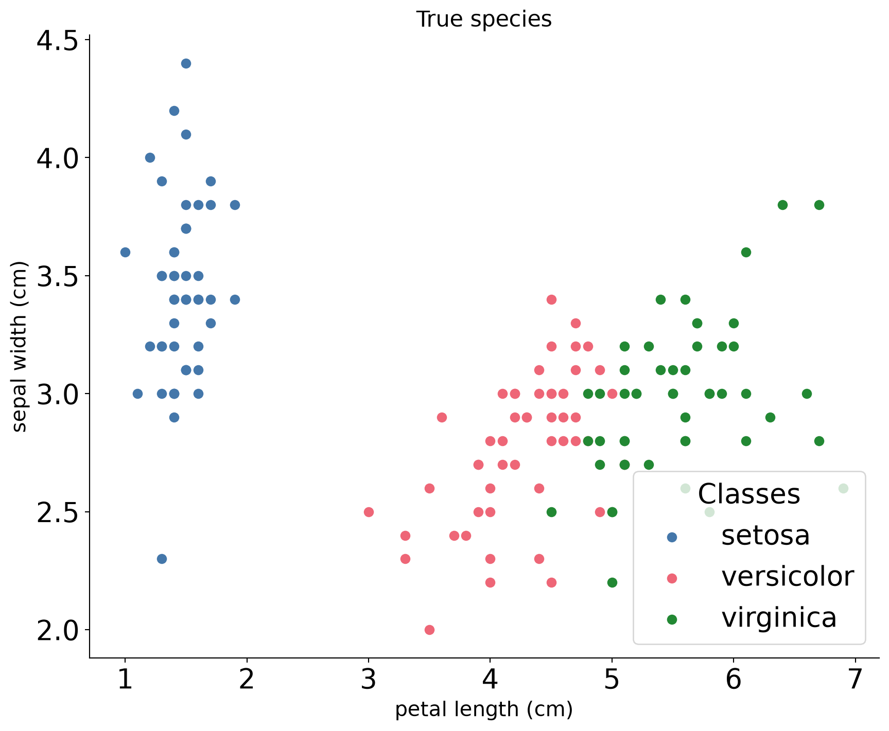
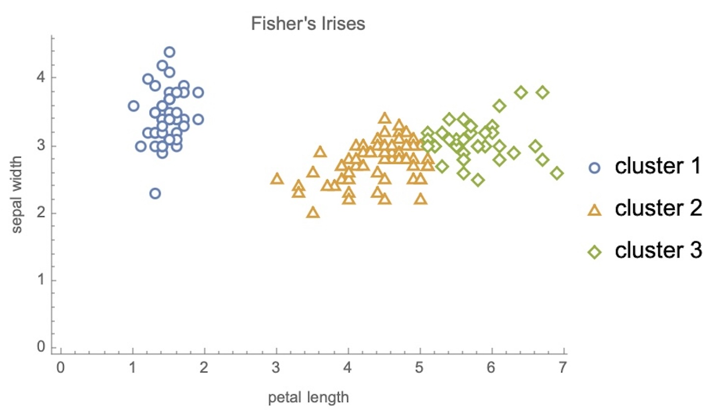
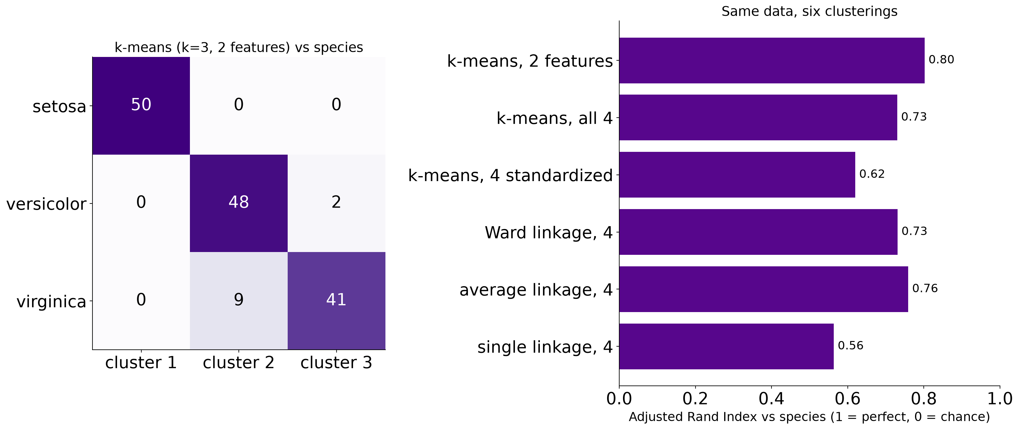
Validating clusters against labels
How many clusters? Two criteria, two answers
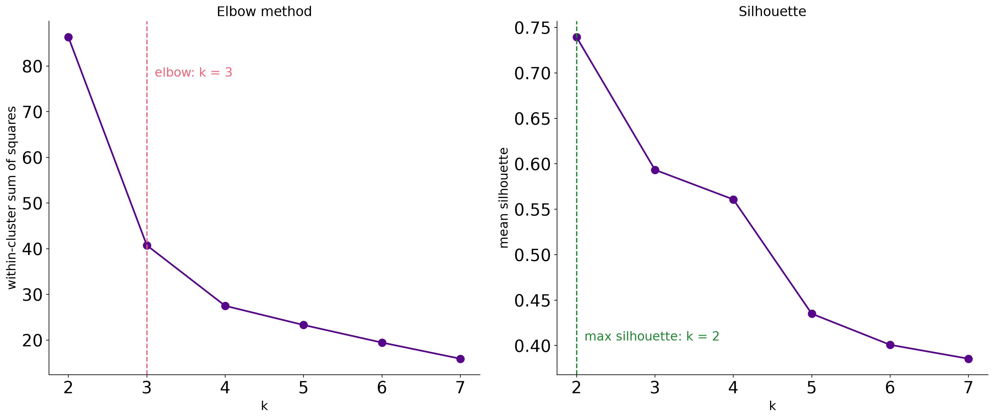
The elbow says 3, the silhouette says 2, the botanist says 3.
Hierarchical clustering: the dendrogram
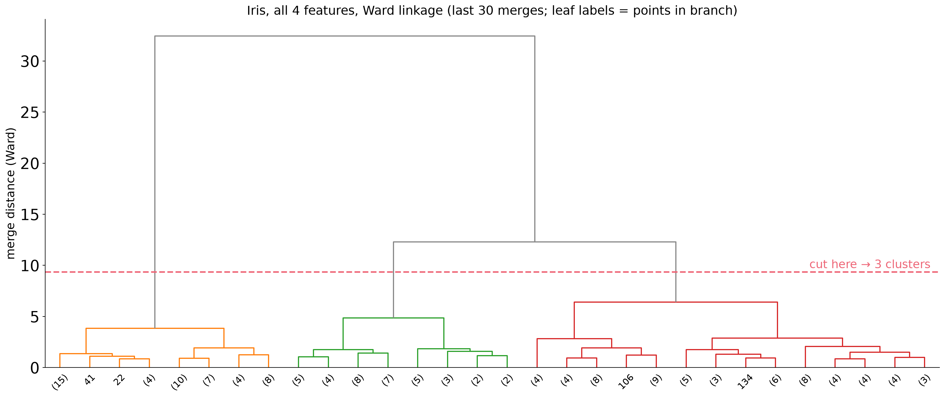
One tree, every k: the cut height is the choice.
Cluster IDs are arbitrary: the colors mean nothing
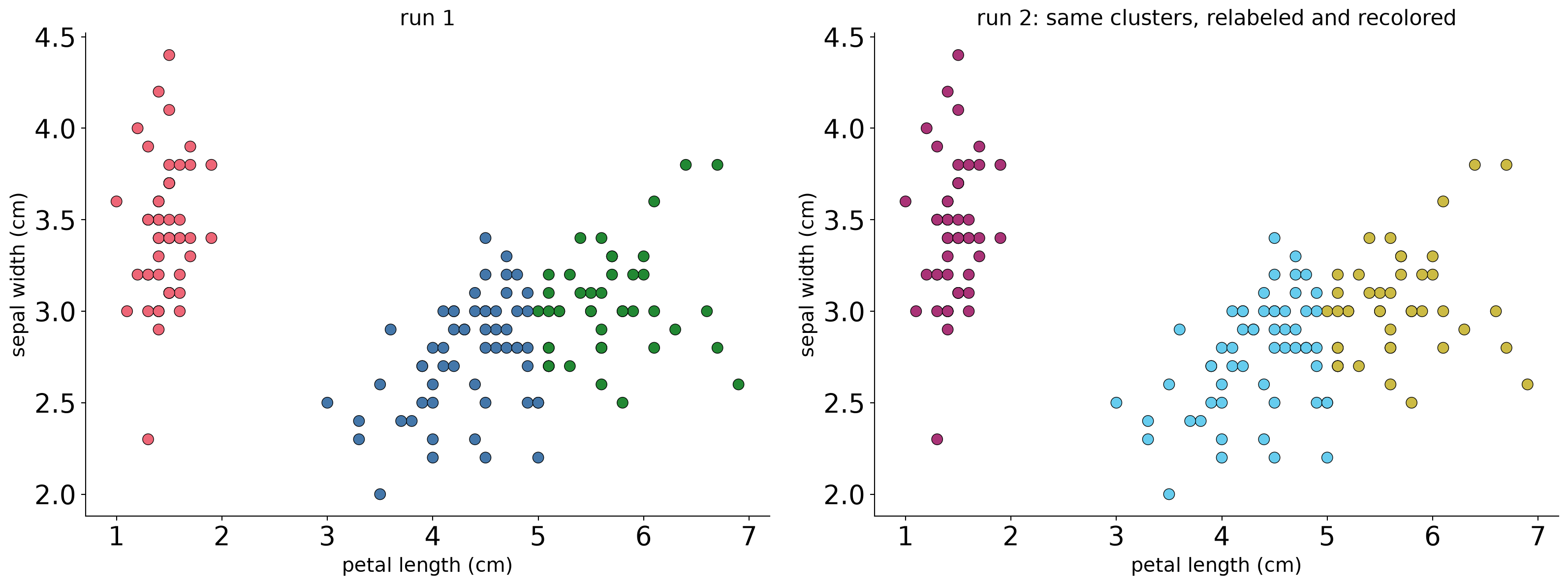
Same partition, different picture. Colors should not suggest an order or a meaning the clusters don’t have.
Seeing the whole tree: clustered heatmap
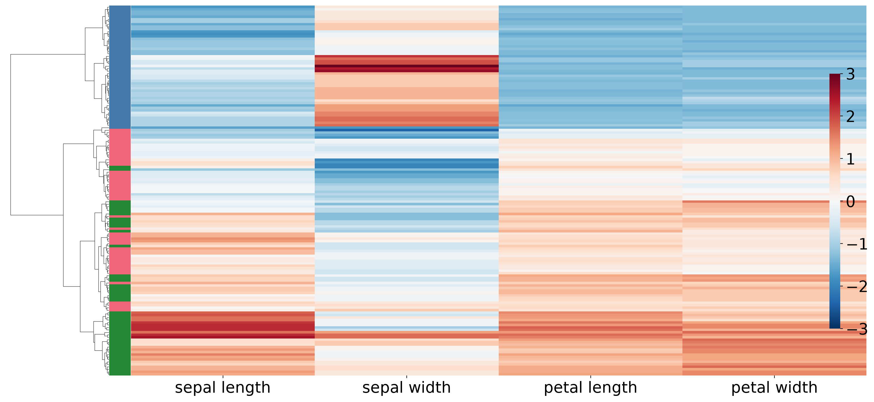
Rows are flowers, columns are measurements, the tree reorders the rows. The side bar is the species, held out.
Per-point quality: the silhouette plot
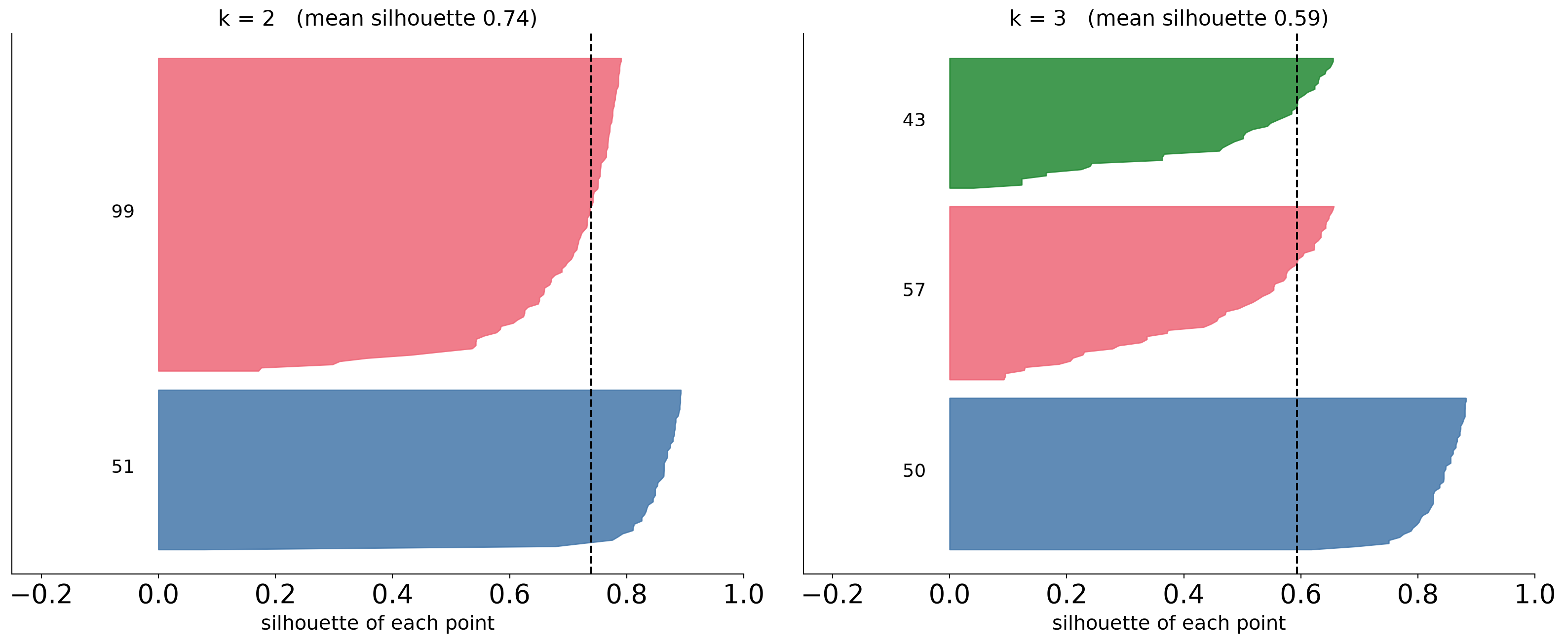
One bar per point, grouped by cluster. Thin or negative bars are points that may be in the wrong place.
Dimensionality Reduction
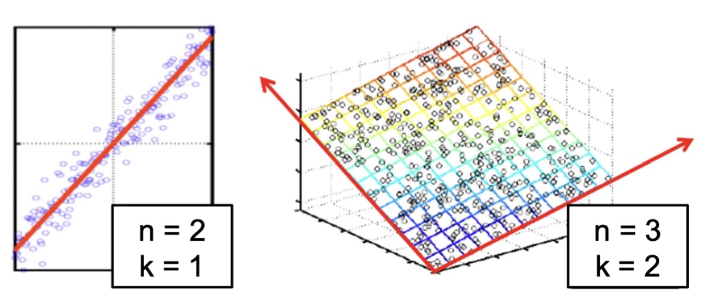
Assumption: data lies on a lower dimensional space
Visualizing the Manifold Hypothesis: Images of ‘3’ Perturbed by Non-linear Operations

What operations did we perform? What’s the intrinsic dimensionality?
Here the underlying manifold is non-linear
Principal Component Analysis: intuition
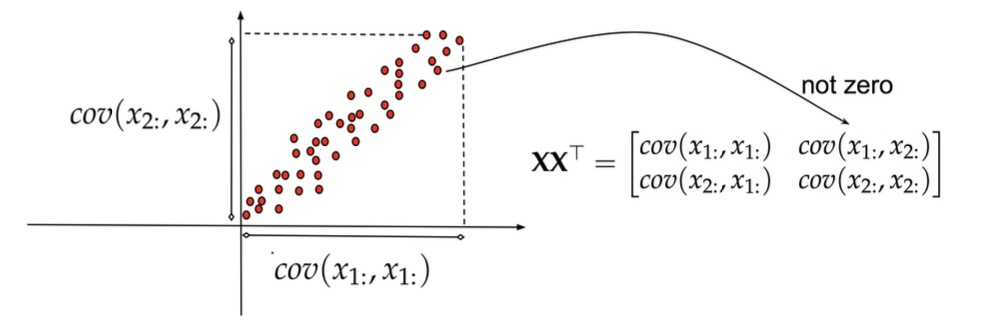
Principal Component Analysis: intuition
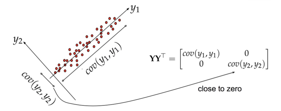
Principal Component Analysis
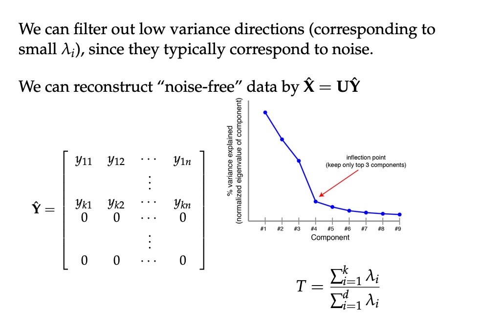
Principal Component Analysis
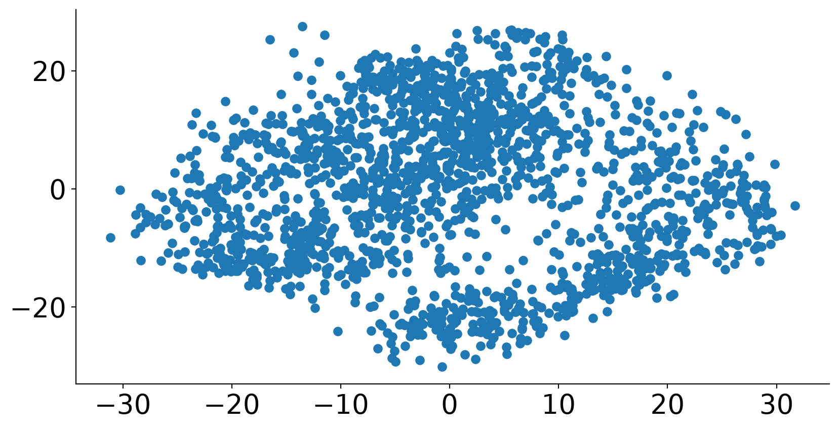
PCA of digits
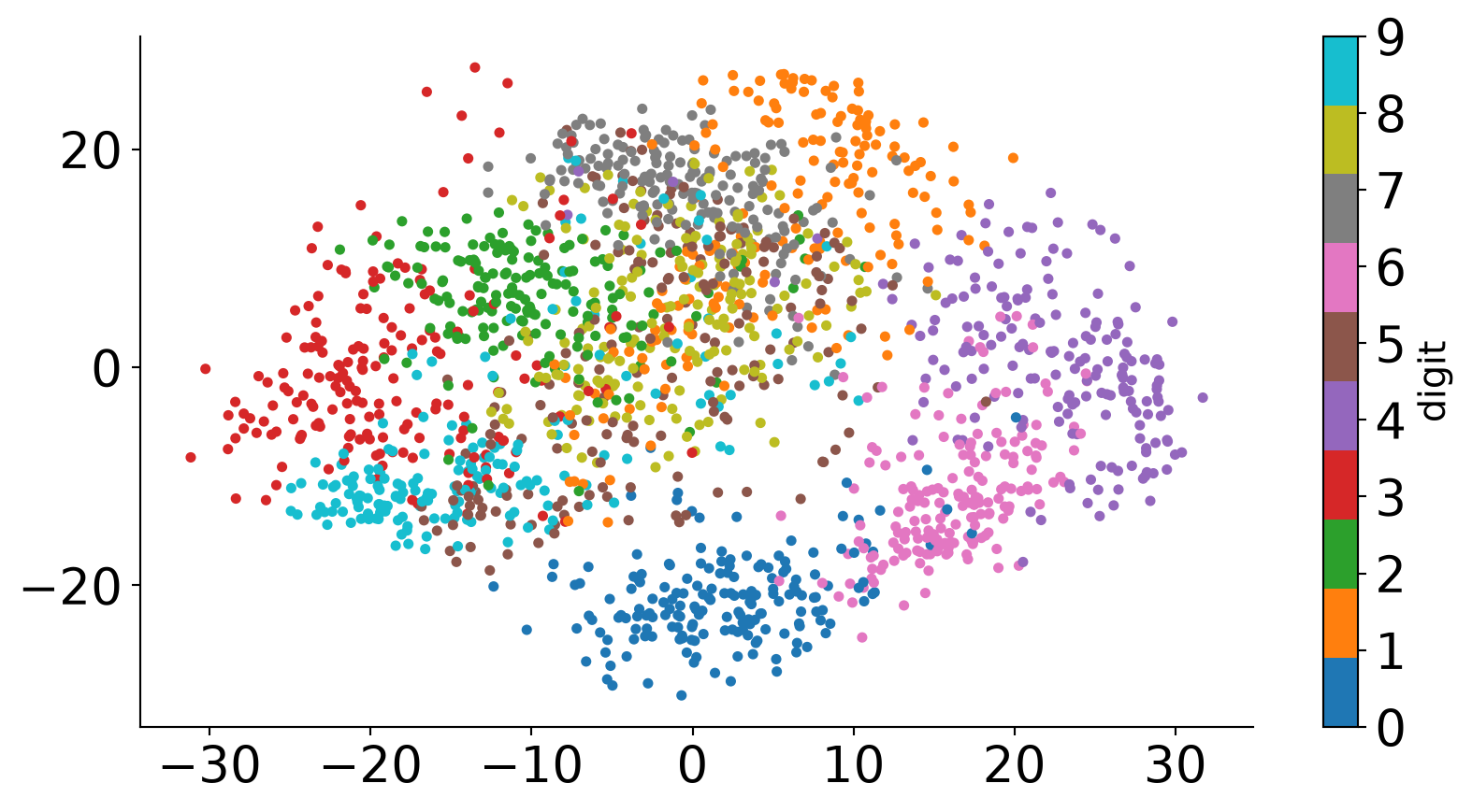
PCA of digits
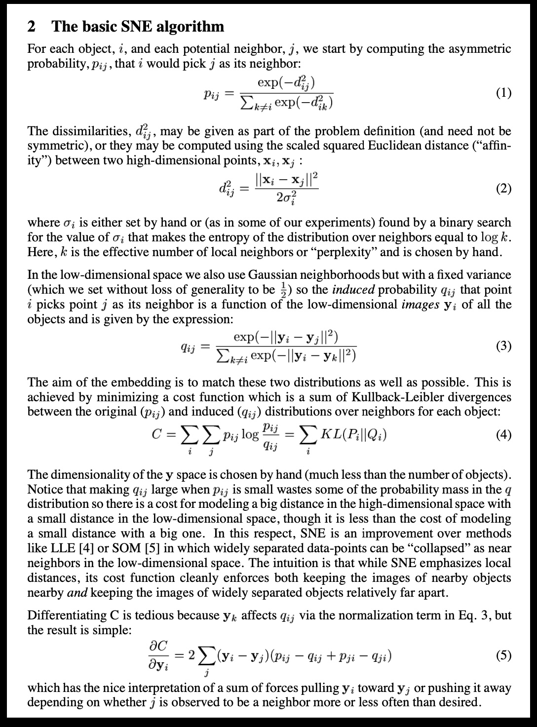
SNE and t-SNE
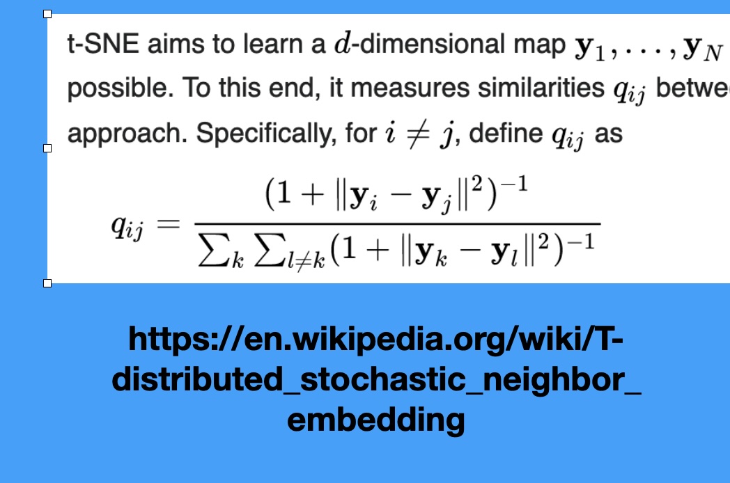
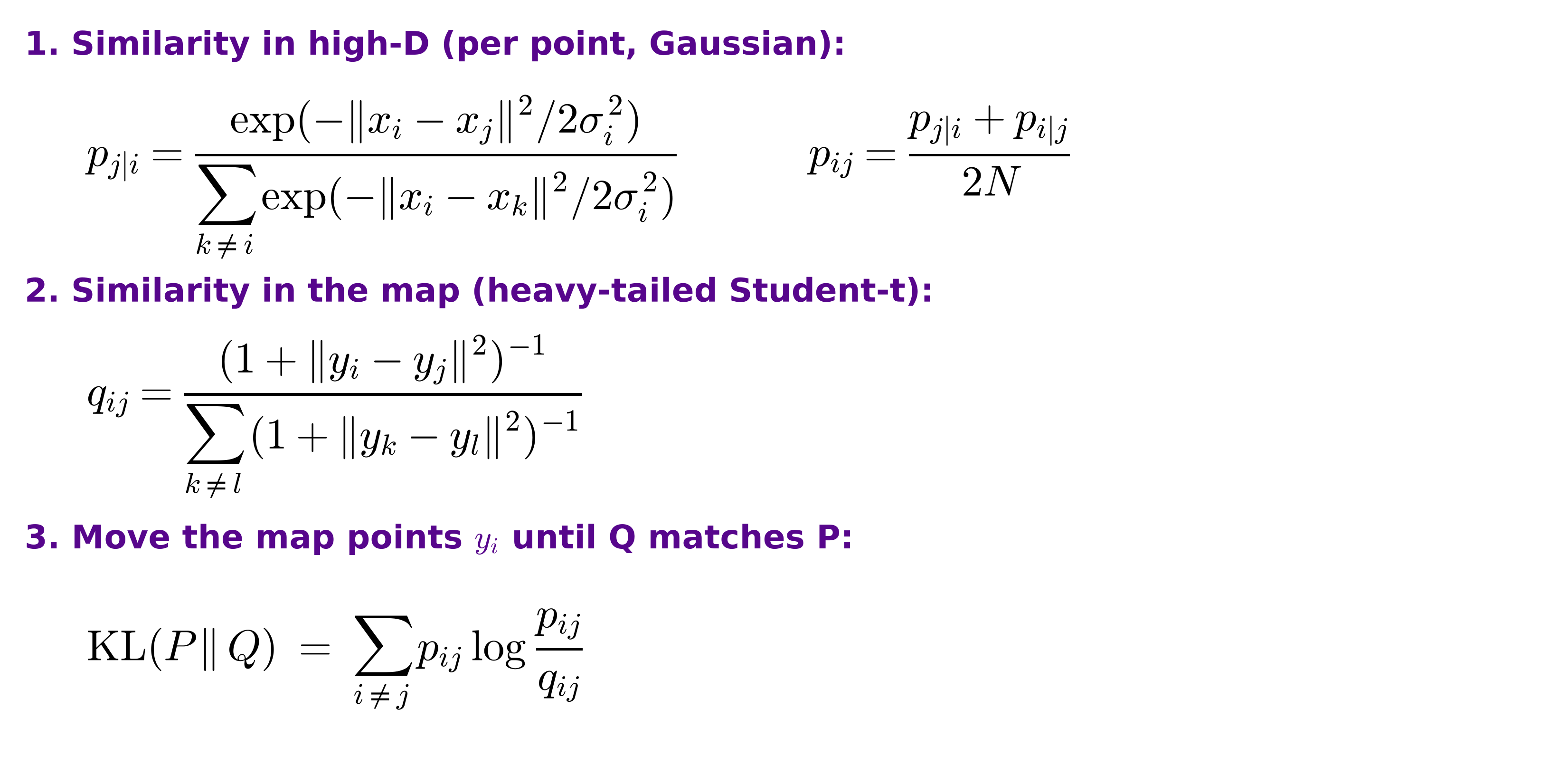
t-SNE in three steps
Why a heavy tail? The crowding problem
- In high dimensions a point can have many neighbors that are all about equally far from it. In 2-D there is not room for them
- With a Gaussian in the map (SNE), moderately distant pairs look very dissimilar, so the optimizer pulls everything into one crowded blob
- The Student-t tail decays polynomially: pairs at moderate distance can sit far apart in the map at almost no cost, which opens gaps between clusters
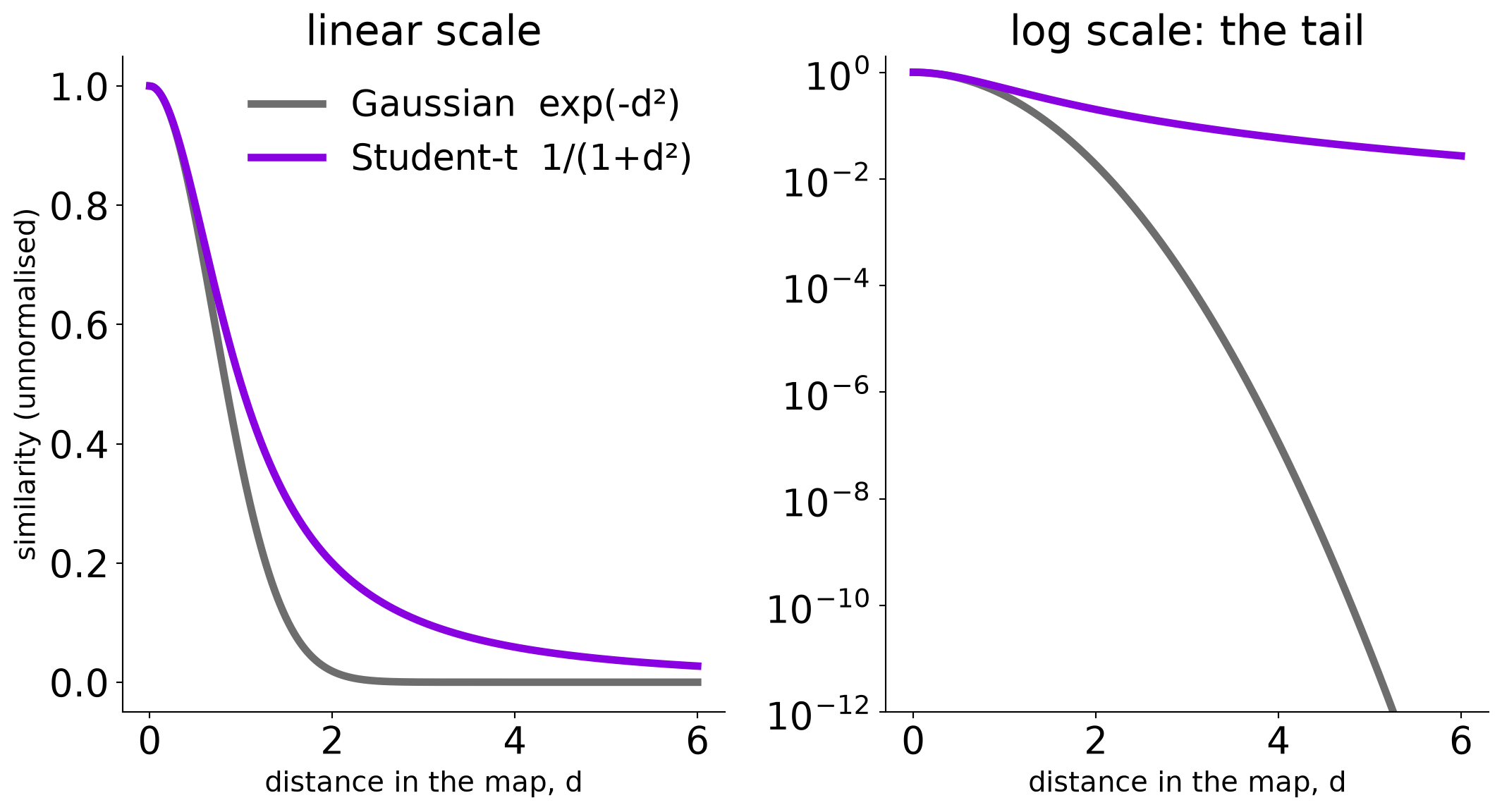
Illustrative kernels: Gaussian vs Student-t (1 degree of freedom), both scaled to 1 at distance 0.
Wattenberg, Viégas, and Johnson, 2016
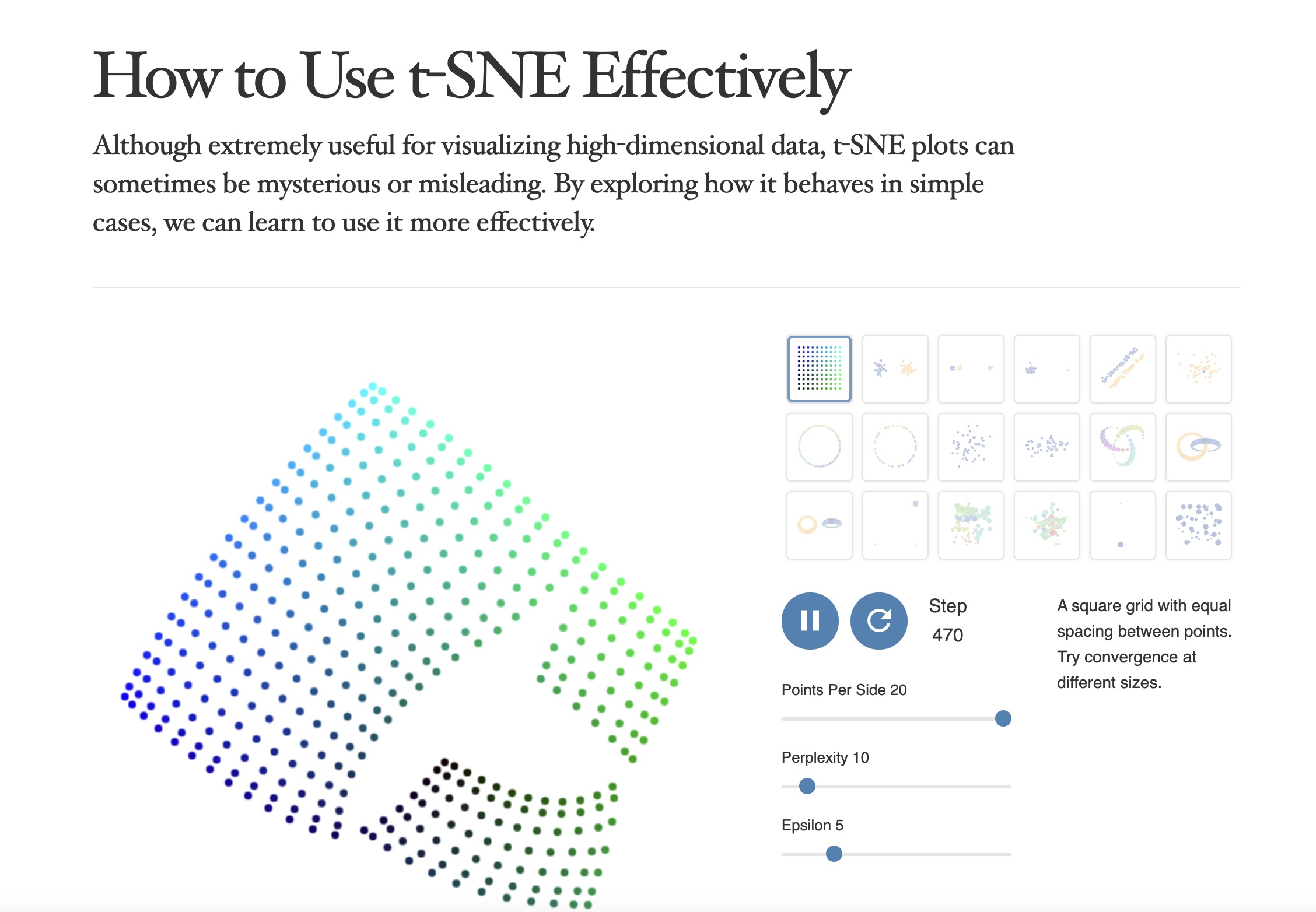
https://distill.pub/2016/misread-tsne/
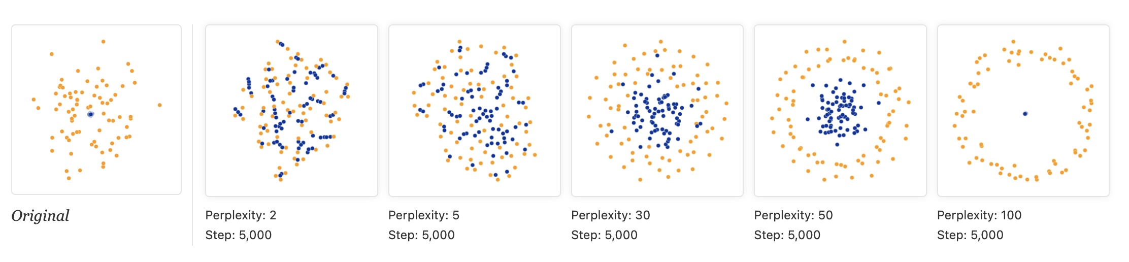
t-SNE
- “Those hyperparameters really matter”
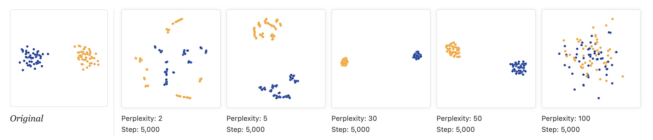
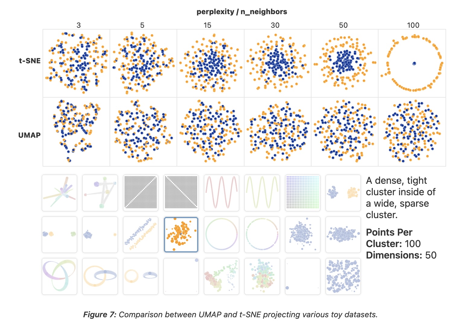
- “The image for perplexity 100, with merged clusters, illustrates a pitfall: for the algorithm to operate properly, the perplexity really should be smaller than the number of points.”
Try it: perplexity on 1,797 digits
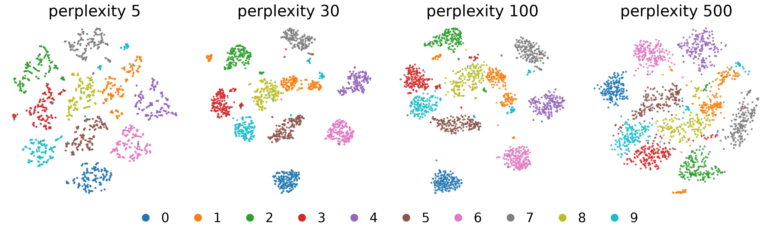
- Same data and seed; only the perplexity changes
- At 5 the groups are loose and fragmented; 30 and 100 give ten clear groups; at 500 (more than a quarter of the dataset) they press into each other
- Which groups end up next to each other changes from panel to panel
t-SNE
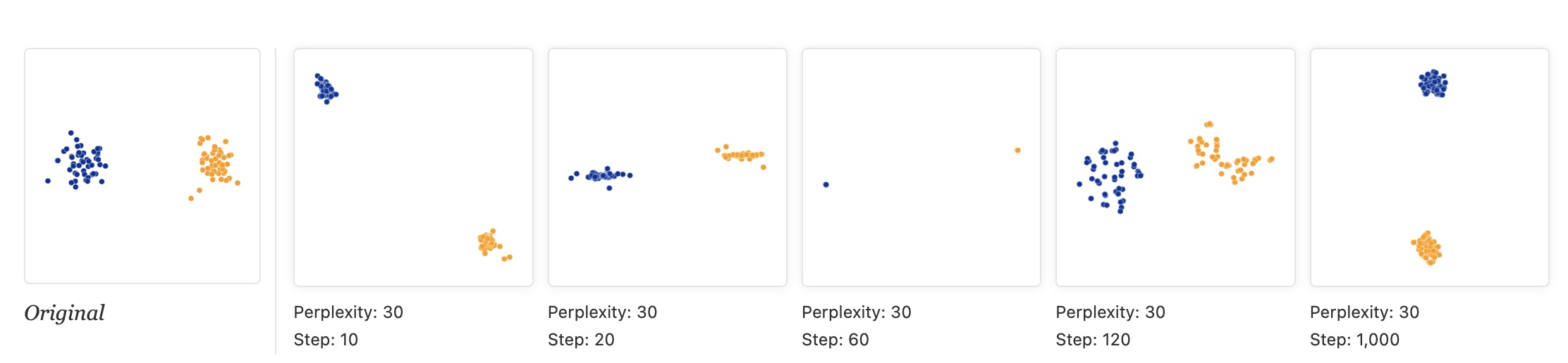
- “Each of the plots above was made with 5,000 iterations with a learning rate (often called “epsilon”) of 10, and had reached a point of stability by step 5,000. How much of a difference do those values make?”
t-SNE
- “Cluster sizes in a t-SNE plot mean nothing”
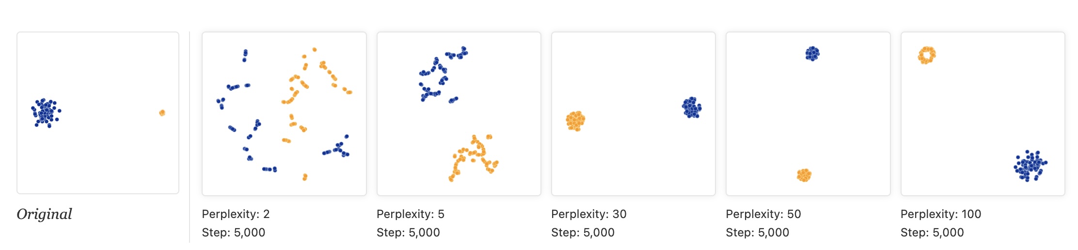
“Size refers to spatial extent/area, not the number of points in the cluster.”
“The t-SNE algorithm adapts its notion of”distance” to regional density variations in the data set. As a result, it naturally expands dense clusters, and contracts sparse ones, evening out cluster sizes.”
t-SNE
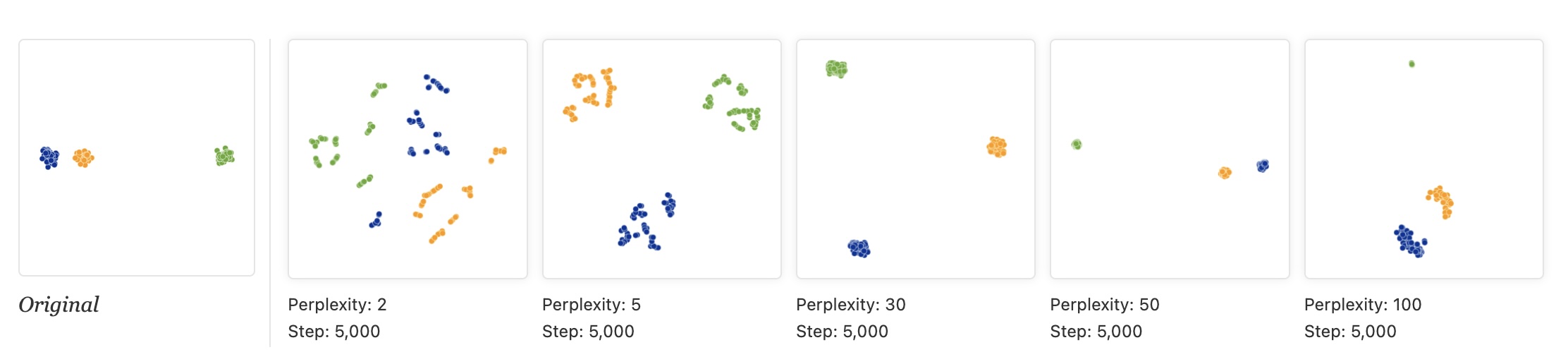
“Distances between clusters might not mean anything”
“The next diagrams show three Gaussians of 50 points each, one pair being 5 times as far apart as another pair.”
Try it: same perplexity, different random start
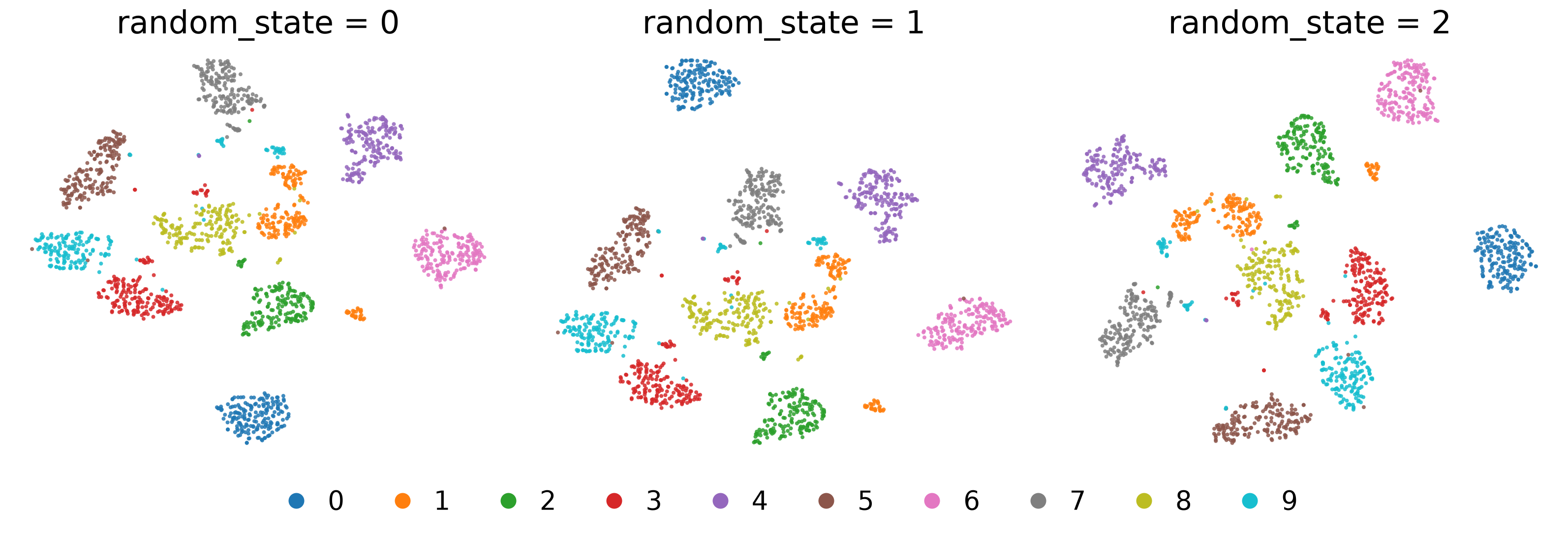
- Same data, same perplexity (30), random initialization; only the seed changes
- The same ten groups appear each time, but the arrangement changes
- Digit 0 (blue) sits at the bottom, the top left, and the far right
t-SNE
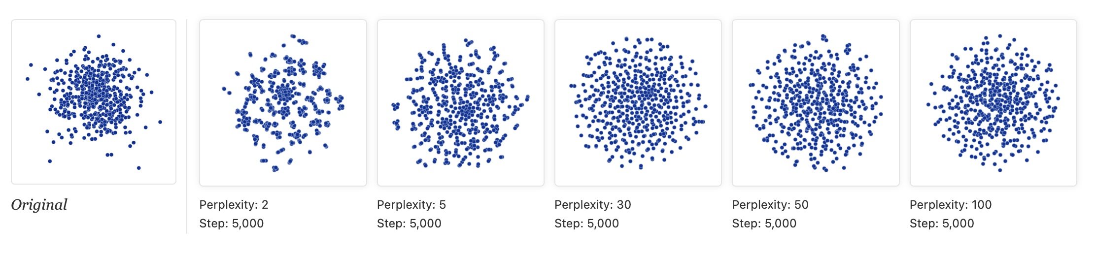
“Random noise doesn’t always look random.”
“The next diagrams show genuinely random data, 500 points drawn from a unit Gaussian distribution in 100 dimensions. The left image is a projection onto the first two coordinates.”
t-SNE
“For topology, you may need more than one plot”
“The plots below show two groups of 75 points in 50 dimensional space. Both are sampled from symmetric Gaussian distributions centered at the origin, but one is 50 times more tightly dispersed than the other. The “small” distribution is in effect contained in the large one.”
Topomap (Doraiswamy et al)
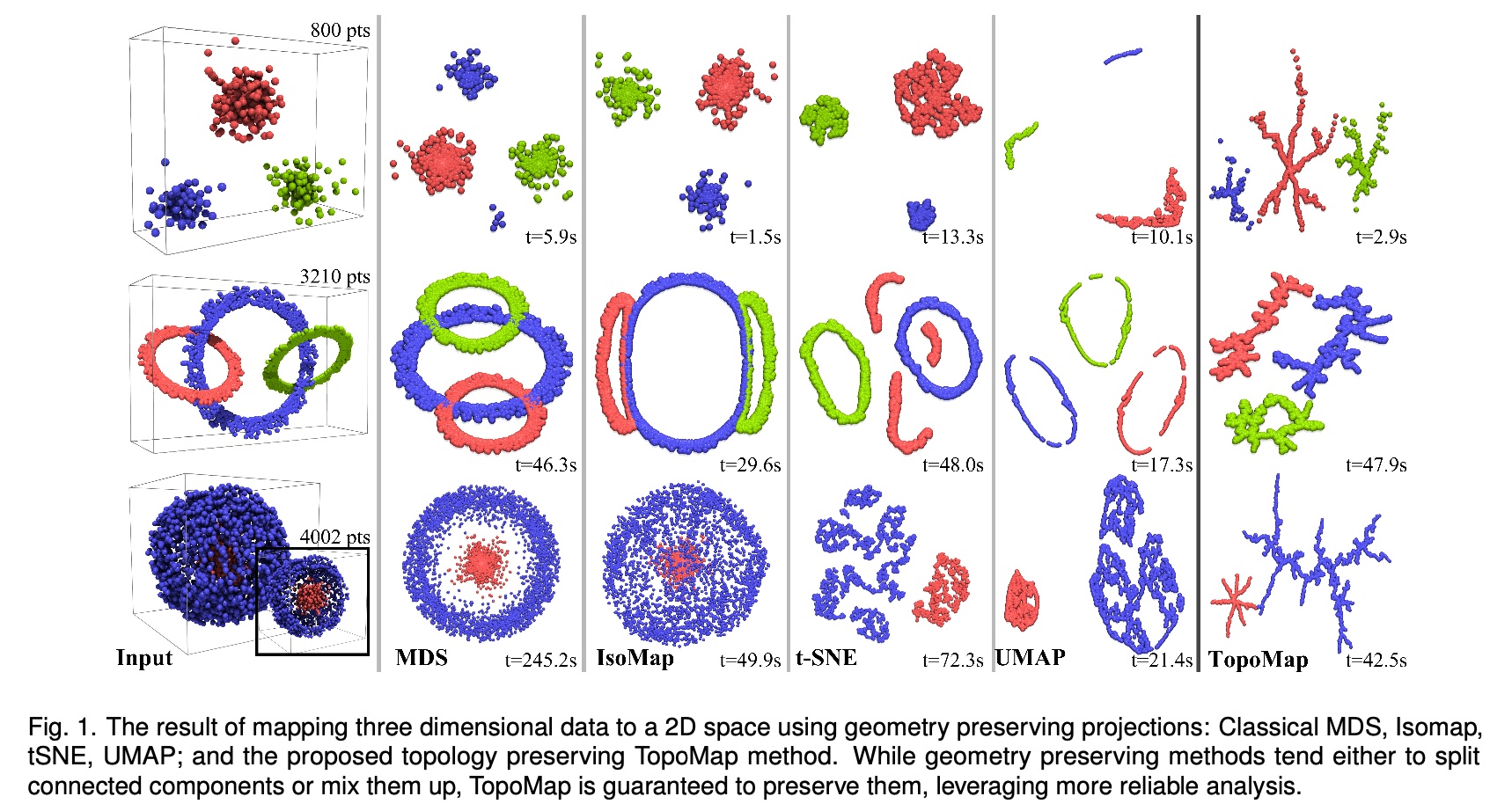
- Topomap preserves the 0-dimensional persistence diagram of the Rips filtration of the high-dimensional data.
Understanding UMAP (Coenen & Pearce)
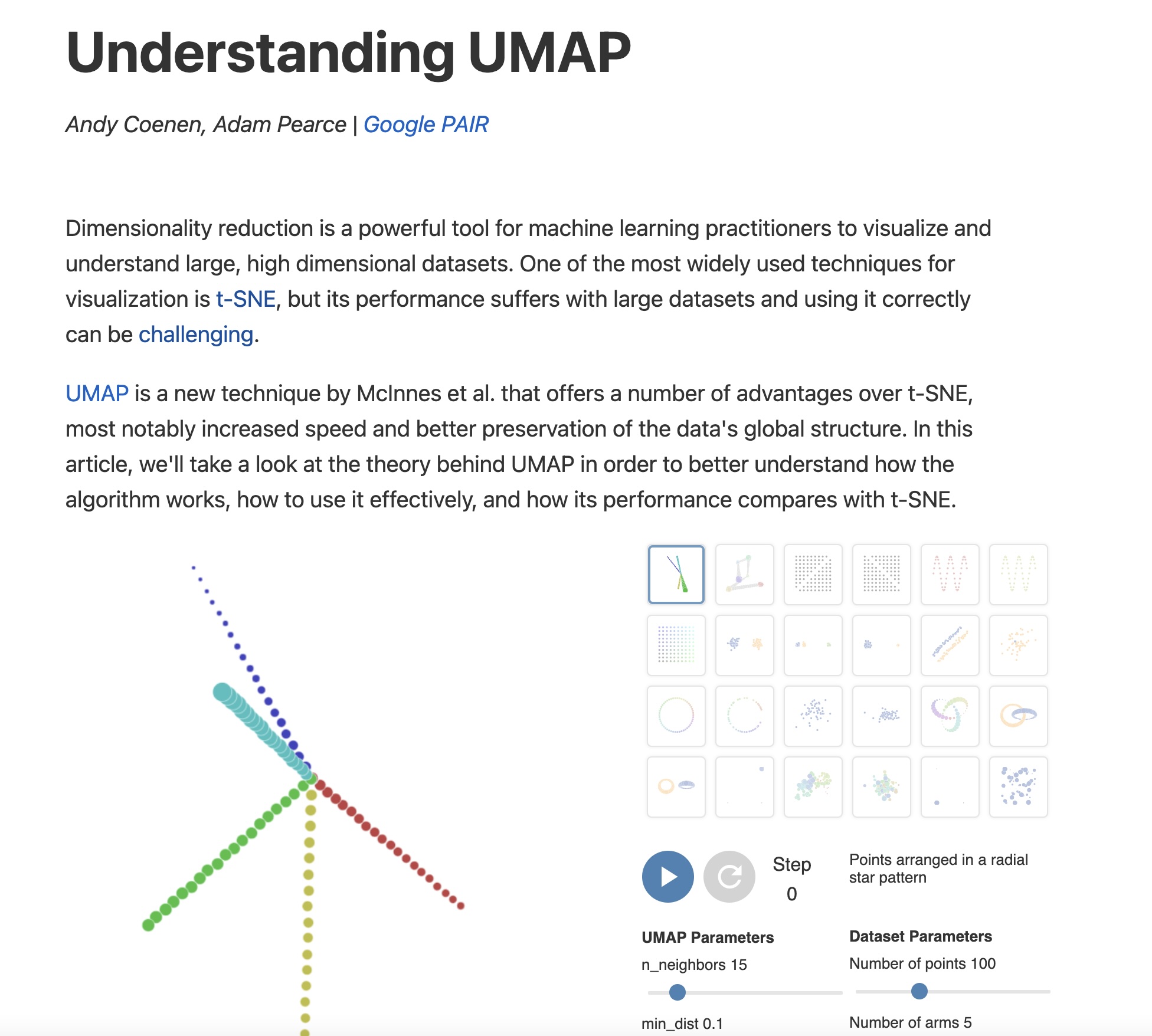
https://pair-code.github.io/understanding-umap/
UMAP
- Coenen and Pearce: “UMAP is fast, scaling well in terms of both dataset size and dimensionality. … UMAP can project the 784-dimensional, 70,000-point MNIST dataset in less than 3 minutes, compared to 45 minutes for scikit-learn’s t-SNE implementation. Additionally, UMAP tends to better preserve the global structure of the data.”
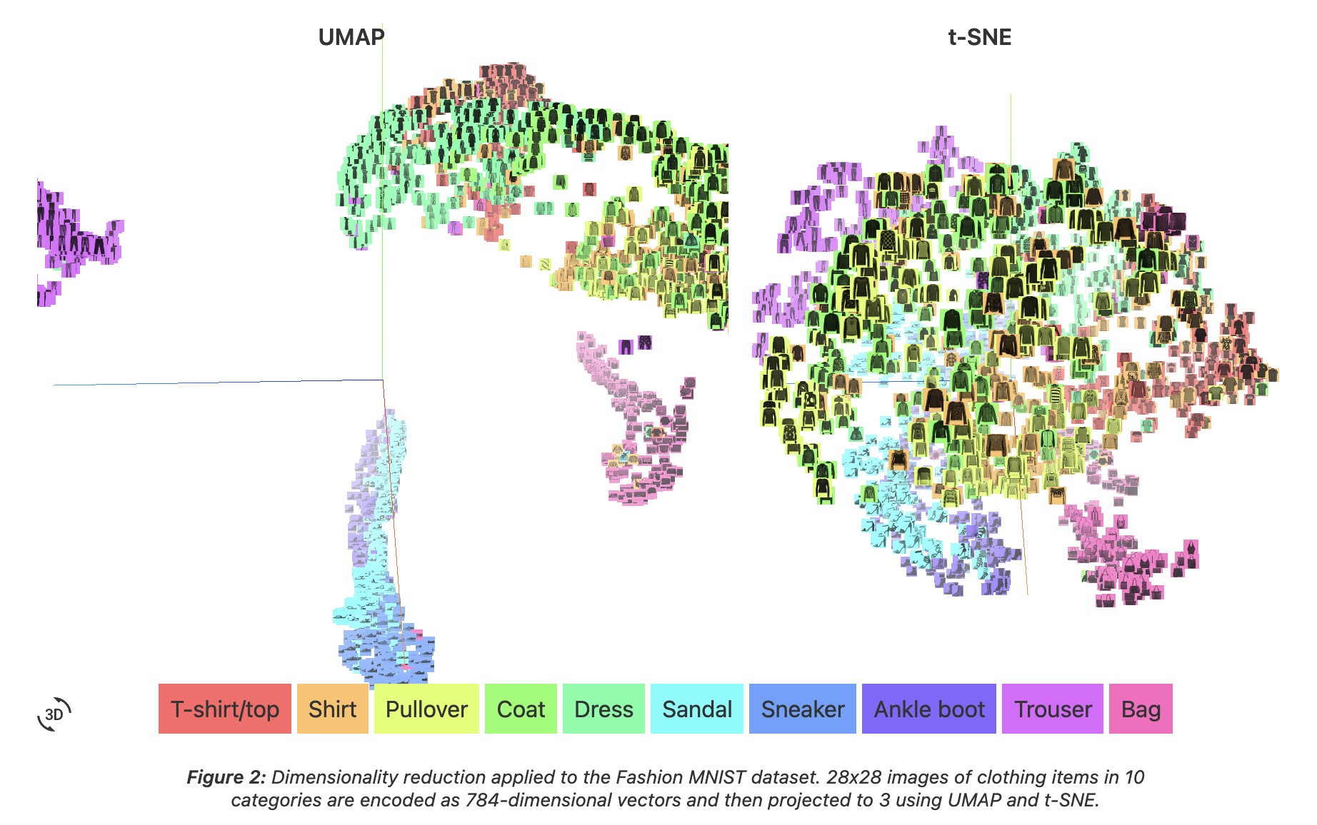
UMAP
- “UMAP, at its core, works very similarly to t-SNE - both use graph layout algorithms to arrange data in low-dimensional space.”
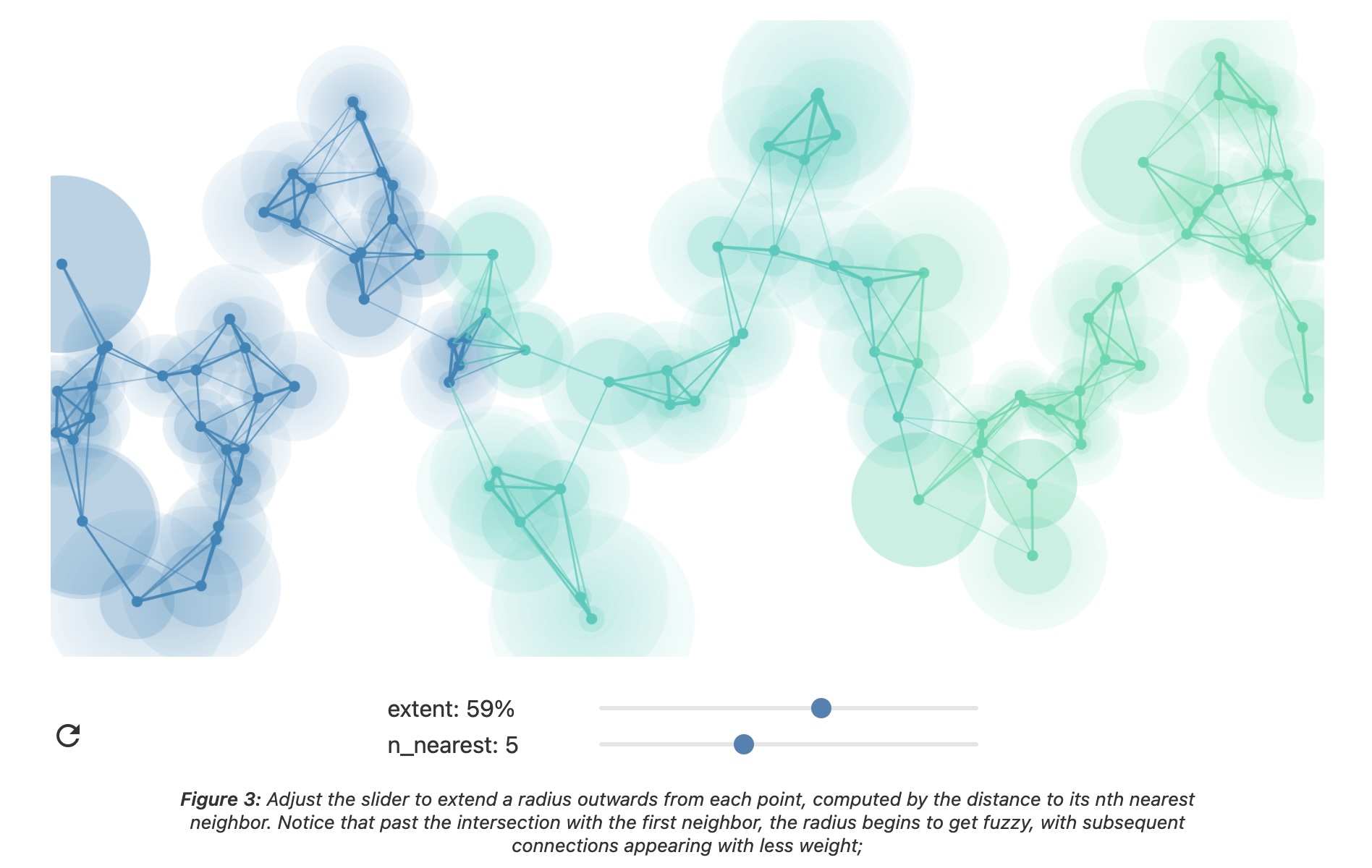
UMAP parameters
n_neighbors - the number of approximate nearest neighbors used to construct the initial high-dimensional graph.
min_dist - the minimum distance between points in low-dimensional space.
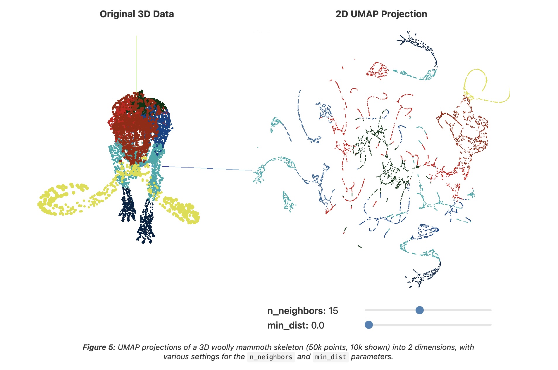
UMAP parameters
n_neighbors - the number of approximate nearest neighbors used to construct the initial high-dimensional graph.
min_dist - the minimum distance between points in low-dimensional space.
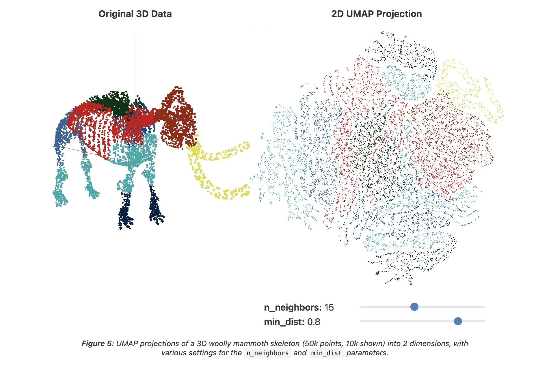
Try it: UMAP n_neighbors × min_dist
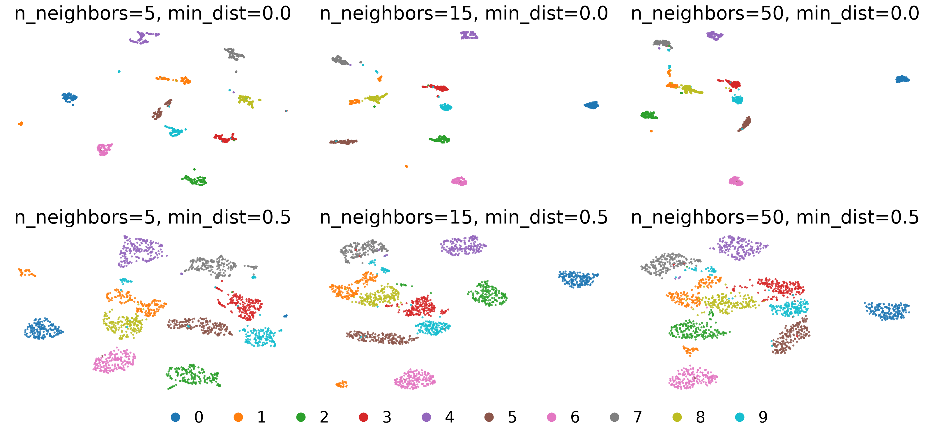
- Rows: min_dist 0.0 vs 0.5. Columns: n_neighbors 5, 15, 50. min_dist changes how tightly points pack; n_neighbors changes how the groups are laid out relative to each other
UMAP
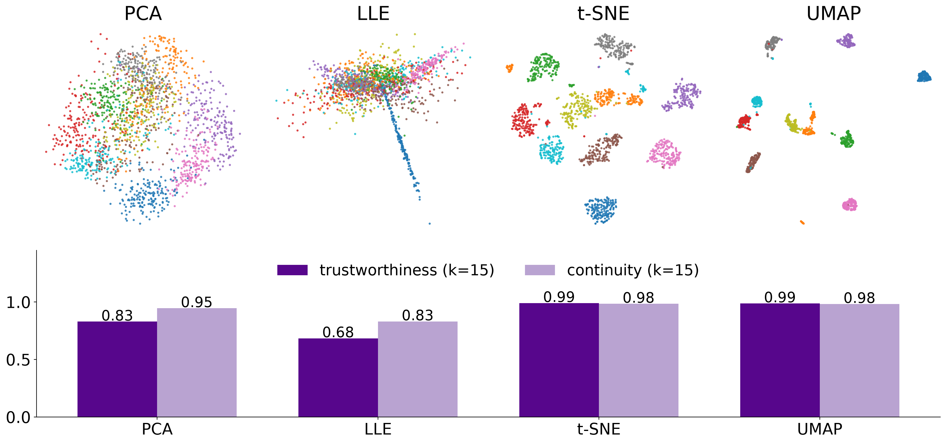
Four projections of the digits, scored
But the score barely moves with perplexity
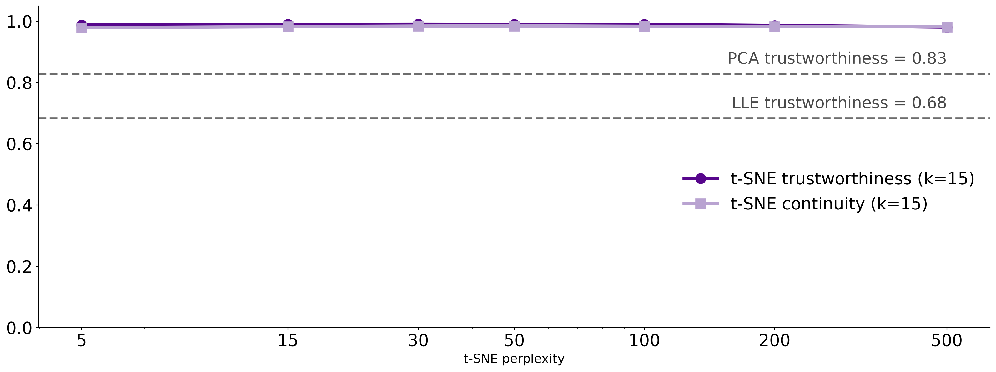
- Perplexity 5 to 500 stays between 0.98 and 0.99, although the maps on the earlier slides look quite different. The metric separates methods (dashed lines: PCA, LLE) but is too coarse to pick a perplexity, and it cannot see cluster sizes or the gaps between clusters
What about user interaction?