Introduction
Based on materials by Enrico Bertini
LECTURE TIMING GUIDANCE (150 min total)
This is a PACKED lecture with lots of content. Suggested timing:
Core Material (90-100 min): MUST COVER - Intro + Temporal Data Fundamentals (15 min): Types, structures, aggregation - Line Charts + Aspect Ratio + Banking to 45° (20 min): Cleveland’s research - Multiple Lines + Spaghetti Plots + Solutions (15 min): Critical problem - Small Multiples transition to Interaction (20 min): Zoom, brushing & linking - Area Charts + Baseline Bias (10 min): Another critical limitation - Event Data + Gantt Charts (10 min): Practical techniques
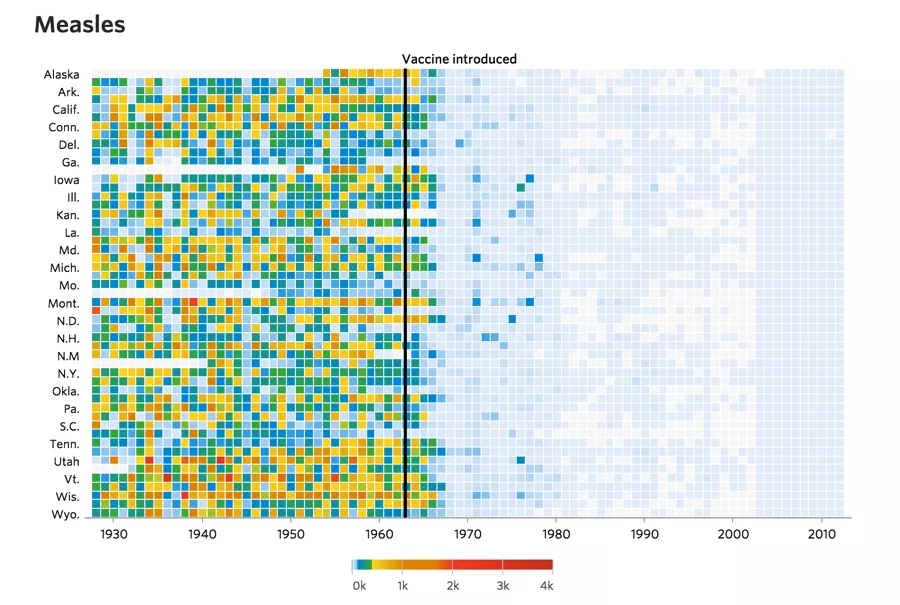
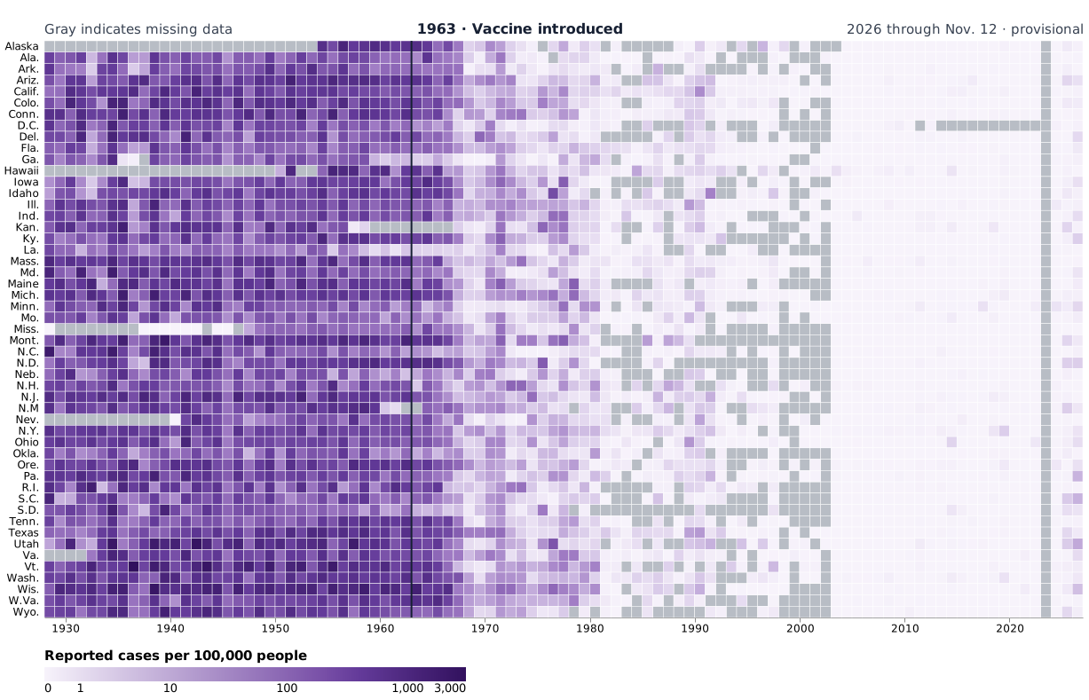
Important but Optional (30-40 min): COVER IF TIME PERMITS - Heat Maps + WSJ Vaccine Example (15 min): Famous example, worth showing - Calendar Visualizations (10 min): Students will use these - Radial Layout Warnings (5 min): Important cautionary note
Advanced/Optional (20-30 min): READING ASSIGNMENT IF SHORT ON TIME - Spiral Plots (5 min) - Horizon Charts (15 min): Complex technique, needs slow walkthrough - Sparklines (5 min) - Alternative Encodings (5 min)
Strategy if running short: 1. Skip Spiral Plots entirely 2. Show Horizon Charts as “further reading” 3. Make sure to cover Banking to 45°, Spaghetti Plots, Baseline Bias (core perceptual issues)
Why Does Time Matter?
SKIPPABLE opener (new for 2026, shared with the VisML deck).
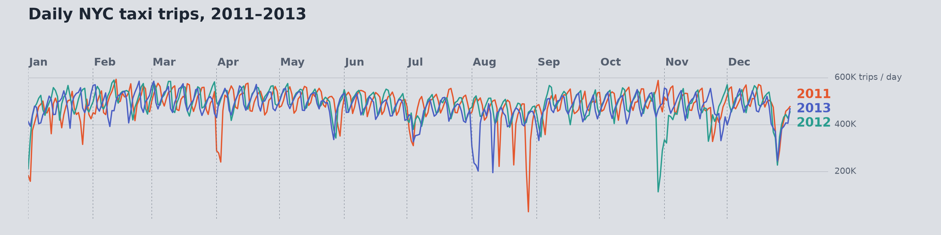
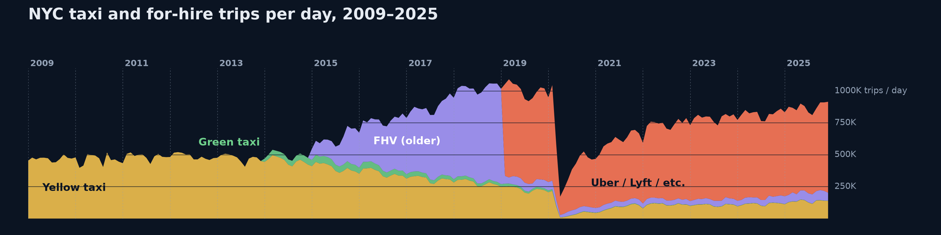
Ask what a single average of daily trips would hide.
Top: three years aligned by calendar date. The weekly rhythm repeats and a few days drop sharply (holidays, storms). That is a cyclic structure plus events.
Bottom: zoomed out to 2009-2025, the mix of services shifts (yellow, green, then for-hire vehicles such as Uber and Lyft) and there is the sharp drop in 2020. That is a sequential structure.
Careful reading: the purple-to-orange switch in 2019 is mostly a reporting change (the TLC began publishing high-volume for-hire trips, i.e. Uber/Lyft, as their own category in Feb 2019), not a jump in service. A good example of a data-definition change showing up as a pattern in time.
Callback to Week 9 (TaxiVis): the same taxi data, now read only along time.
Transition: “Both charts are the same kind of data. What makes data temporal?”
What is Temporal Data?
Definition : Data in which values depend on time and time is explicitly recorded.
In other words: we track when things happened or what values were at specific points in time
This is a fundamental concept - time is not just an attribute, it’s THE organizing dimension
START WITH THIS QUESTION : “What datasets have you used or seen that have time in them?”
Get 3-4 student examples on the board
For each example, ask: “How is time recorded? What’s the granularity?”
Emphasize that temporal data requires explicit time recording - not just “ordered” data
Common misconception: Students often think any sequential data is temporal (e.g., ranking lists)
Key distinction: Temporal data has meaningful time stamps/intervals, not just ordering
Example: Temporal Dataset Structure
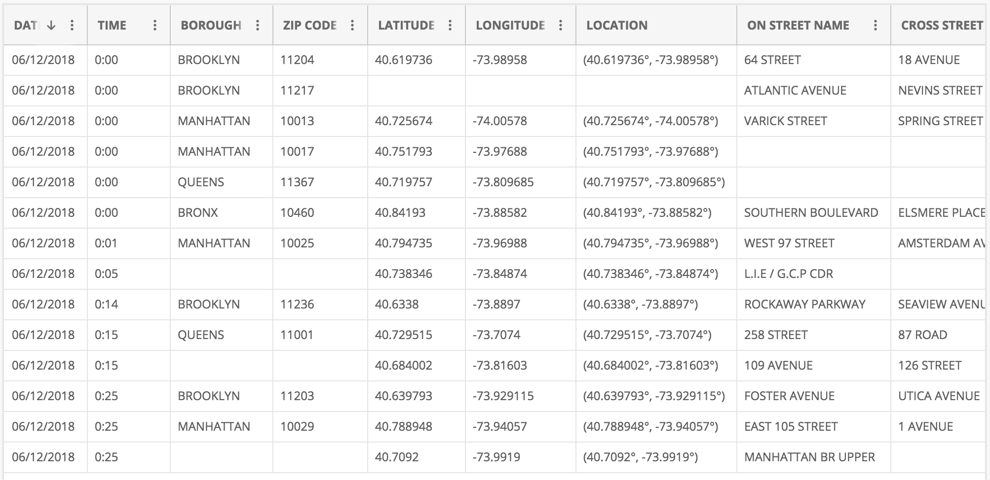
The DATE and TIME columns make each collision record temporal data.
Each row is one incident/event at a specific location and time, so we can ask when, where, and how often
These are NYC motor vehicle collision records (NYC Open Data): borough, ZIP, lat/long, street names. The first header reads DAT only because the column is truncated in the screenshot
PHYSICALLY POINT to the DAT and TIME columns on screen with mouse/pointer
“See these columns? This is what makes this temporal data - explicit timestamps”
Make sure image is zoomed/large enough for back row to see
Note the other attributes (location, type) that we might want to analyze over time
Questions to pose: “What patterns might we want to find? Daily patterns? Seasonal? Hot spots over time?”
Wait for answers - students might suggest: “crime by hour of day”, “seasonal trends”, “geographic patterns over time”
This is event data (discrete occurrences) rather than continuous measurements
Application Domains
Business
Natural Phenomena
Behaviors/Movement
Traffic/Mobility
Medical/Healthcare
Finance
Temporal data is EVERYWHERE - this is one of the most common data types
Ask students to give specific examples for each domain:
Business: Sales trends, customer activity, website traffic
Natural Phenomena: Weather, earthquakes, climate change
Behaviors/Movement: GPS tracks, social media activity, eye tracking
Traffic/Mobility: Vehicle flow, public transit usage, flight patterns
Medical: Patient vitals, disease progression, treatment outcomes
Finance: Stock prices, trading volume, economic indicators
Emphasize: Different domains have different temporal characteristics (irregular vs regular sampling, event-based vs continuous)
Type 1: Event Data
Time + Object (Attributes)
“Something happened at time T”
Examples: Tweet, Email, Alarm
CRITICAL distinction: Event data represents discrete occurrences at points in time
Events often have irregular timing - they happen when they happen (not sampled at regular intervals)
Each event is an object with attributes (who, what, where, why)
Examples to emphasize:
Tweet: timestamp + user + text + location
Email: sent time + sender + recipient + subject
Alarm: trigger time + sensor + type + severity
Key visualization challenge: How do we show when events occurred and their attributes?
Often visualized as dots, marks, or bars on a timeline
Type 2: Measurement Data
Time + Measure(s)
“This is the value at time T”
Examples: Temperature, revenue, stock value
EXPLICIT CONTRAST WITH TYPE 1 : “Remember Event Data? Tweet, Email, Alarm - something just happened . Measurement data is different - we’re recording a value at each time point.”Measurement data: Continuous or regularly sampled values over time
Unlike events (which happen irregularly), measurements are typically taken at regular intervals
Each measurement records one or more quantitative values at a timestamp
Side-by-side comparison to emphasize :
Event: “Email sent at 3:42 PM” (binary - it happened)
Measurement: “Temperature was 72°F at 3:42 PM” (quantitative value)
Examples to discuss:
Temperature: Recorded every hour → time series of temperature values
Revenue: Daily sales figures → continuous tracking of performance
Stock value: Price sampled every second during trading hours
Key difference from events: We care about the VALUE at each time point, not just that something occurred
Primary visualization: Line charts, area charts - showing how values change over time
This is what most people think of as “time series data”
Time Structures
Three key structures for temporal data:
Sequential - Linear progression over timeCyclic - Repeating patterns (daily, weekly, seasonal)Hierarchical - Nested time resolutions (year/month/day)
Key insight : Most real temporal data has ALL THREE structures simultaneously!
These are the three fundamental ways time can be structured in data
Sequential : Time flows in one direction - useful for showing trends, growth, changes
Example: Company revenue from 2015-2025
Cyclic : Patterns repeat on a regular basis - reveals rhythms and regularities
Example: Traffic by hour of day, sales by day of week, temperature by season
Natural cycles: daily, weekly, monthly, yearly
Hierarchical : Multiple nested time scales - enables drill-down and multi-resolution analysis
Example: Years contain quarters contain months contain weeks contain days
EMPHASIZE THIS POINT : “Most real temporal data has ALL THREE structures simultaneously!”
Example: Website traffic has sequential trends (growing over years), cyclic patterns (weekday vs weekend), and hierarchical structure (hour/day/week/month)
You choose which structure to visualize based on your question
Visualization choice depends on which structure you want to emphasize
Sequential and Cyclic Patterns
Sequential
(Jan 1, … , Dec 31)
Cyclic
(S, M, T, W, T, F, S)
Hierarchical Time Resolutions
Multiple Resolutions
Years
Months
Weeks
Days
Hours
Linking Data Types to Time Structures
Event Data
Time + Object (Attributes)
Sequential: Transaction logs over years
Cyclic: User logins by day of week
Hierarchical: System alerts by hour/day/month
Measurement Data
Time + Measure(s)
Sequential: Stock prices over time (line charts)
Cyclic: Temperature patterns by season
Hierarchical: Revenue by year/quarter/month
Key Insight : Data type + time structure → visualization choice
NOW we can synthesize : You’ve seen Event vs Measurement AND Sequential/Cyclic/HierarchicalThis slide connects the two fundamental concepts: data types AND time structures
Both event and measurement data can have sequential, cyclic, or hierarchical patterns
The combination determines the best visualization approach
Sequential structure → line charts, area charts (show progression)
Cyclic structure → radial layouts, calendars (emphasize repetition)
Hierarchical structure → multi-scale views, drill-down interactions
Ask students: “If you have daily website traffic, what structures might you see?” (Answer: Sequential trend over months, cyclic pattern by day of week, hierarchical hour/day/week)
Aggregation Trade-offs
Benefits of Aggregation
Reduces noise
Shows overall trends
Manageable data size
Clearer patterns
Example : Daily → Monthly averages reveals seasonal trends
Risks of Aggregation
Masks short-term events
Loses extreme values
Can hide critical peaks
Simpson’s Paradox
Example : A 1-hour server outage disappears in monthly view
Design principle : Choose granularity based on the questions you need to answer
Warning : This is Simpson’s Paradox for temporal data - aggregation can completely reverse or hide patterns!
CRITICAL SLIDE - This is Simpson’s paradox for temporal data!Aggregation is necessary (can’t show raw data at finest granularity) BUT dangerous
Benefits are obvious - reduced noise, clearer trends, manageable visualization
But risks are severe - can completely hide important events
Real example to share : Netflix outage for 1 hour affects millions, but disappears in daily/weekly aggregatesAnother example : Daily COVID cases show spikes, but monthly averages smooth them out - which matters for policy?The “right” aggregation depends on your analytical question:
Looking for long-term trends? → Aggregate more
Looking for anomalies/outliers? → Aggregate less
Best practice: Provide interactive controls to change aggregation level
Mention multi-resolution techniques (coming later): horizon charts, overview+detail
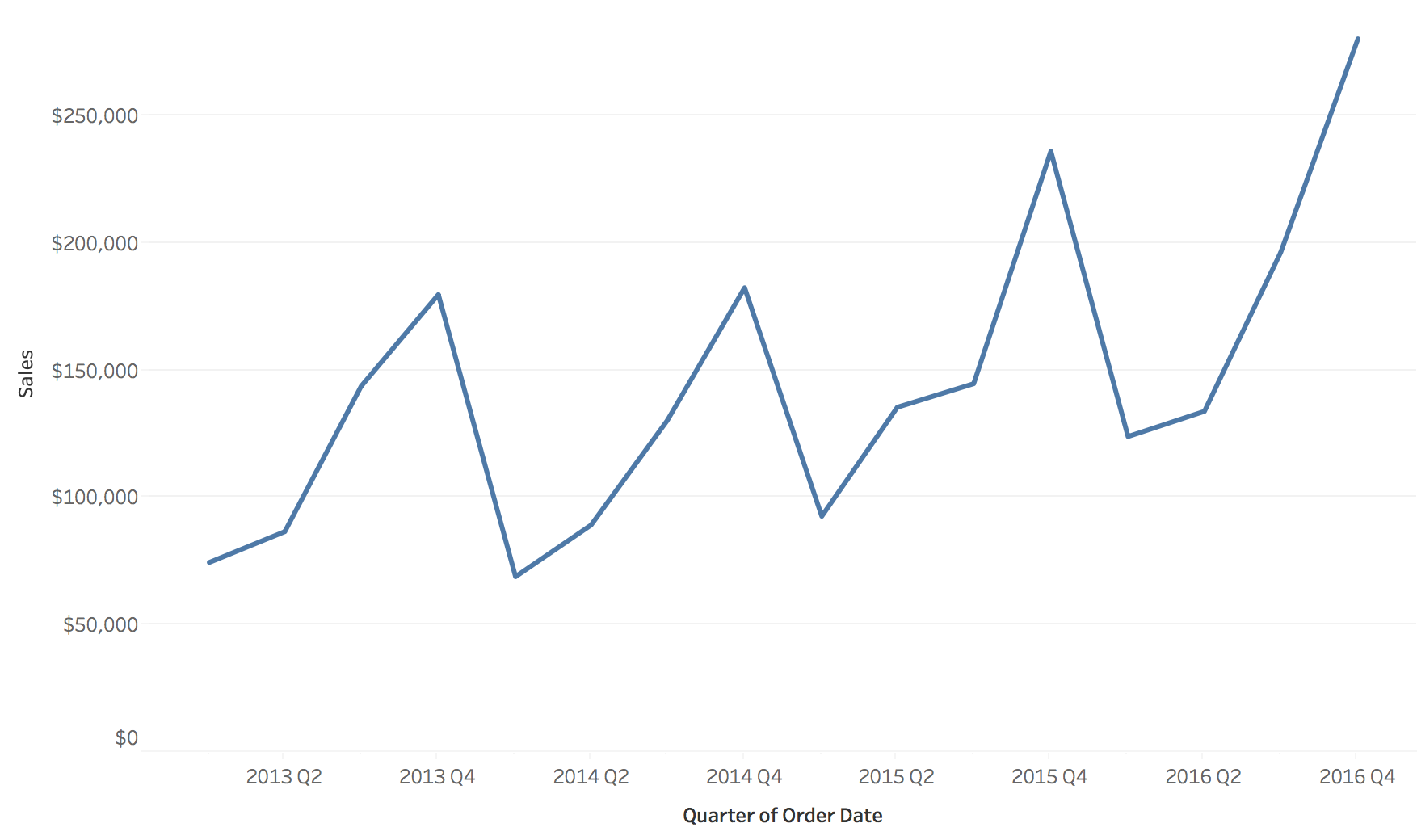
Example: Sales Over Time - Sequential View
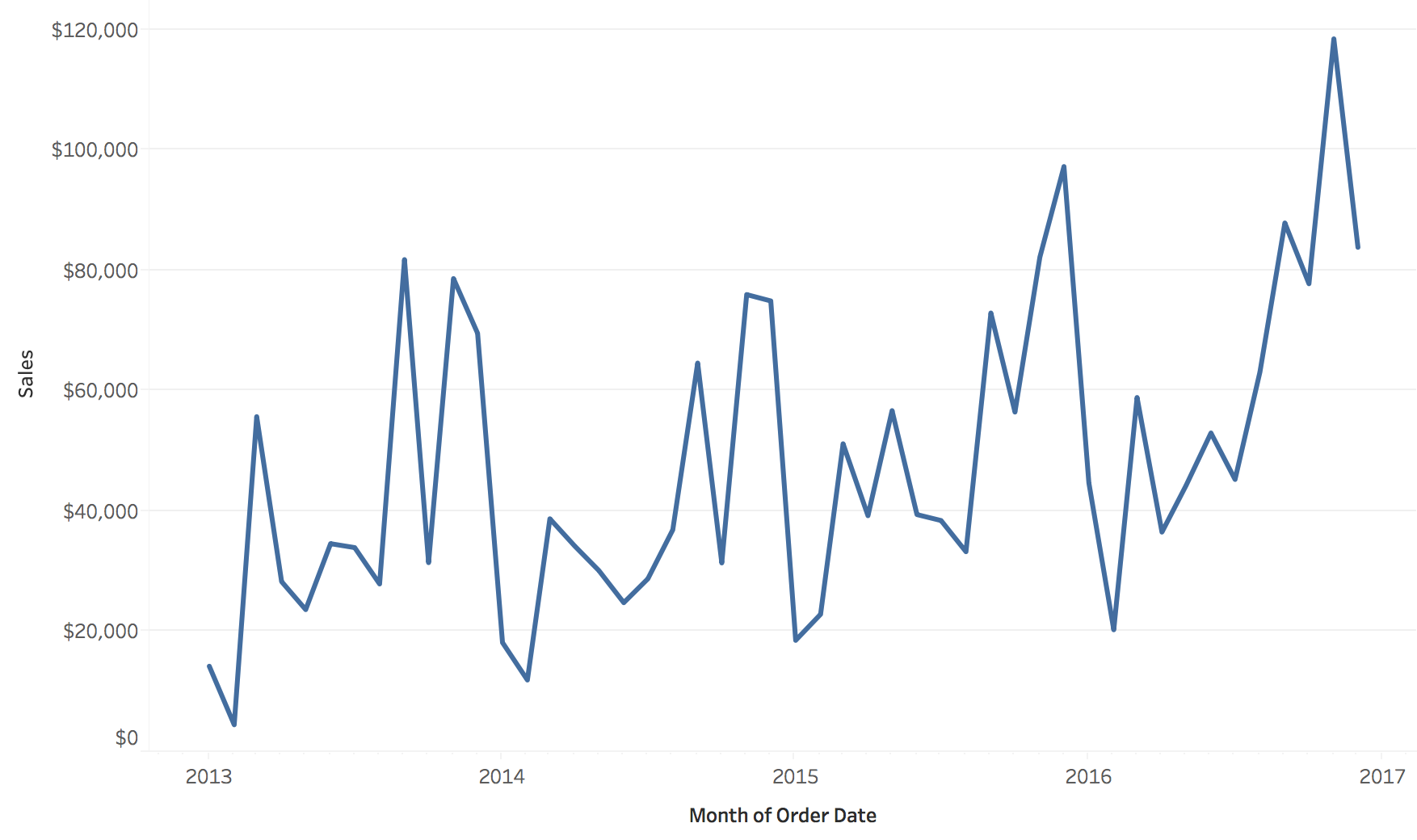
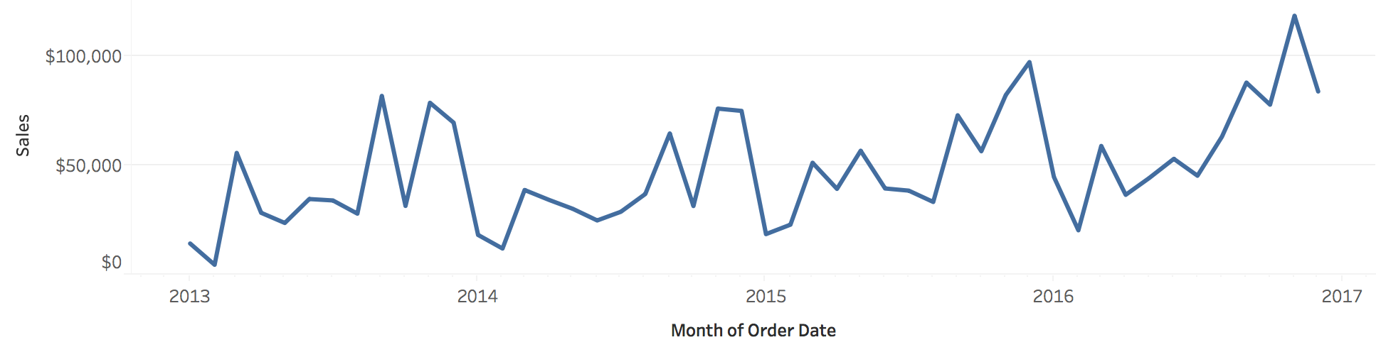
Sequential: “How did our sales change over the years?”
Example: Sales Over Time - Cyclic View
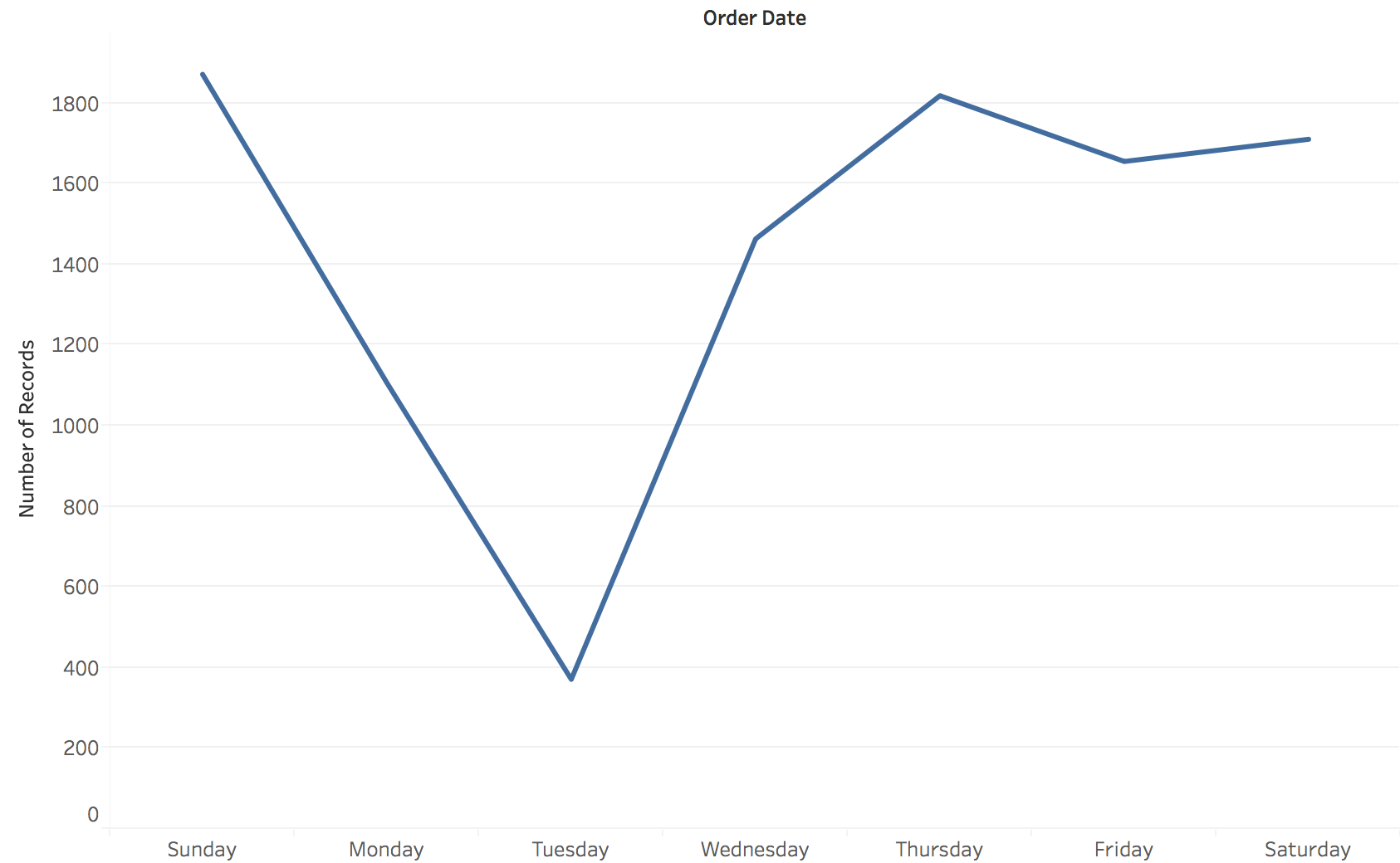
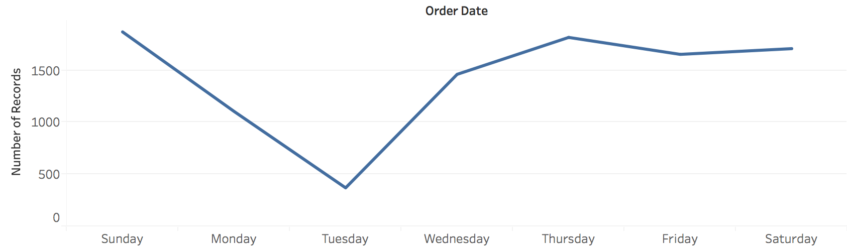
Cyclic: “How does the number of orders change by day of the week?”
Hierarchical Structure and Resolution
Combining multiple time resolutions in one view
Time Resolution: Sequential Views
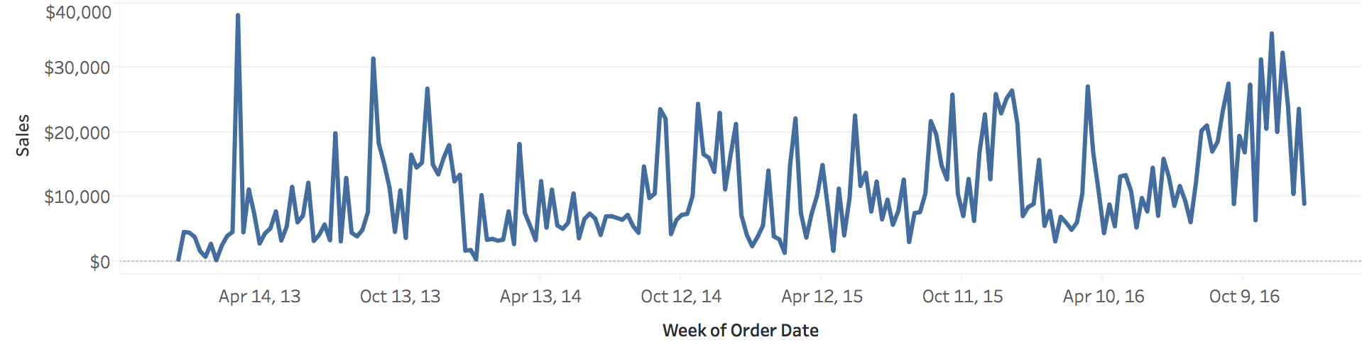
The same sales by week (top) and by month (bottom): granularity changes what you see.
Time Resolution: Cyclic Views
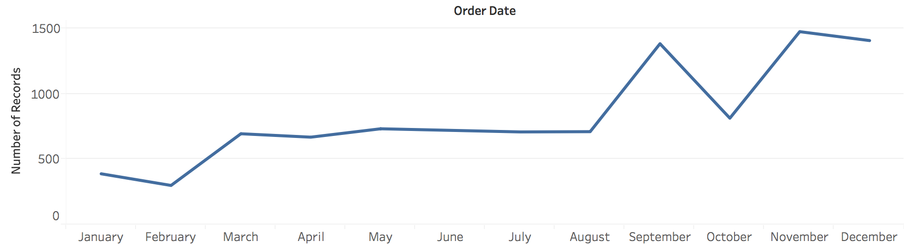
The same orders folded by month of year (top) and by day of week (bottom).
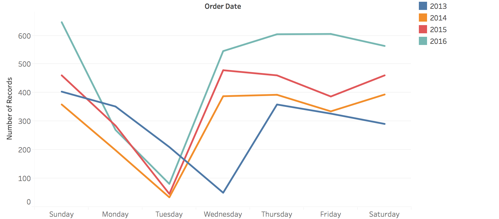
Example: Nesting Cyclic (Day) within Sequential (Year)
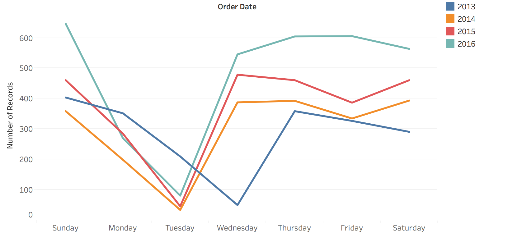
One line per year (2013-2016) across the days of the week: a cyclic view nested in a sequential one.
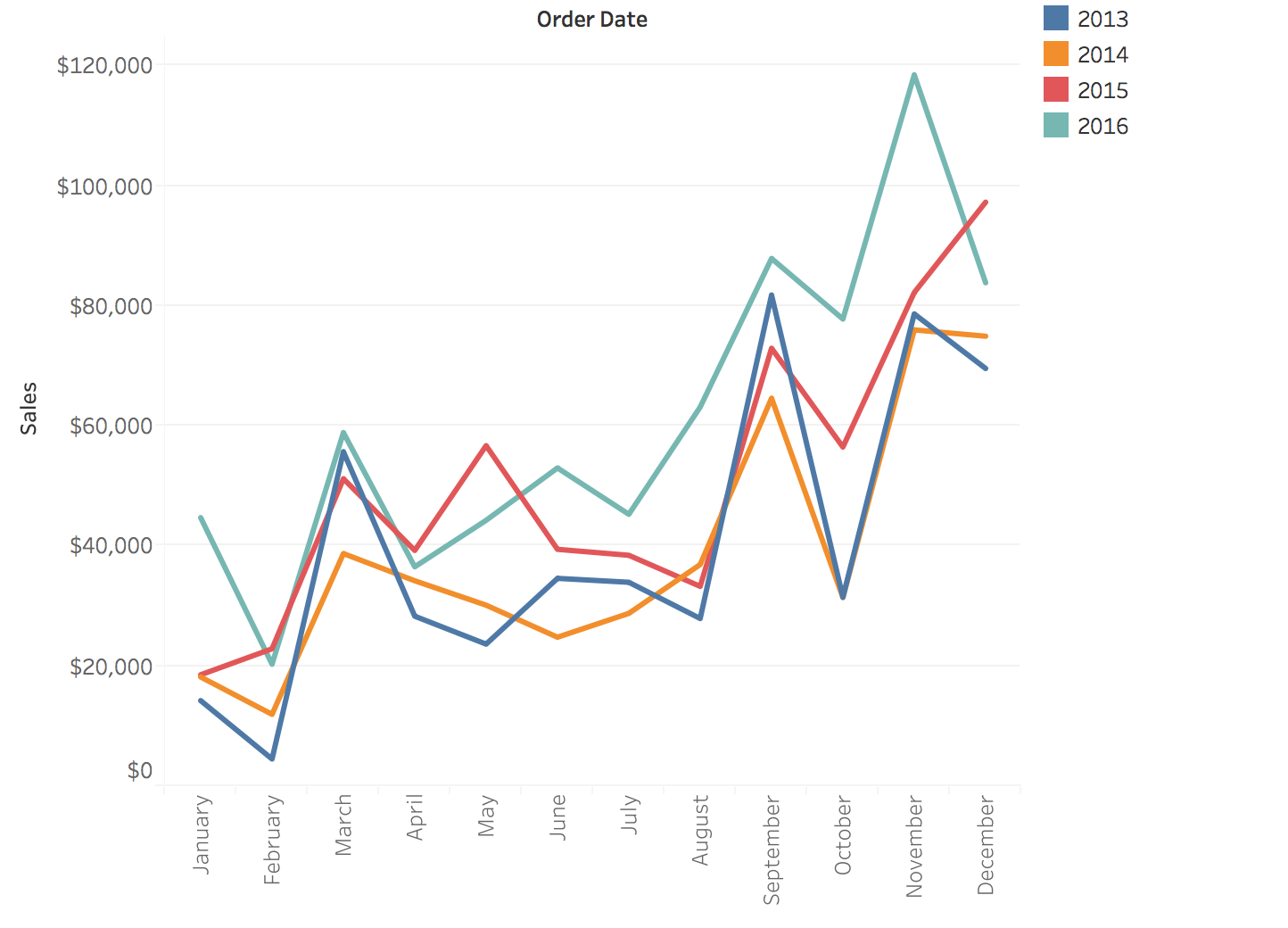
Example: Nested Time Patterns (Monthly)
Sales by month of the year, one line per year (2013-2016).
Aspect Ratio
How chart dimensions affect perception
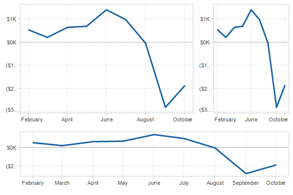
Definition : Aspect Ratio = Width / Height
Impact on Trend Visibility
The same data at three aspect ratios: the trend looks steeper or flatter.
Perceptual Principle: Slope Judgment
Key finding : Humans judge slopes most accurately at 45°
Too shallow (<< 45°): Hard to distinguish small differences
Too steep (>> 45°): Also difficult to compare
Optimal: ~45° - Maximum perceptual sensitivity
This principle guides aspect ratio selection
Fundamental perceptual principle from Cleveland & McGill’s researchOur visual system is optimized for judging slopes near 45 degrees
Demo: Show how very flat lines (<10°) make it hard to see if trend is up or down
Demo: Show how very steep lines (>80°) also make comparison difficult
This isn’t arbitrary - it’s based on empirical perceptual experiments
Practical implication: Don’t just use default aspect ratios from your plotting library!
The aspect ratio is a design parameter that affects what viewers perceive
Ask: “Which stock would you invest in based on this chart?” - then show same data with different aspect ratio revealing different impression
Banking to 45°
Method : set the aspect ratio so that the average slope of the line segments is 45°
Makes trends perceptually salient and comparable
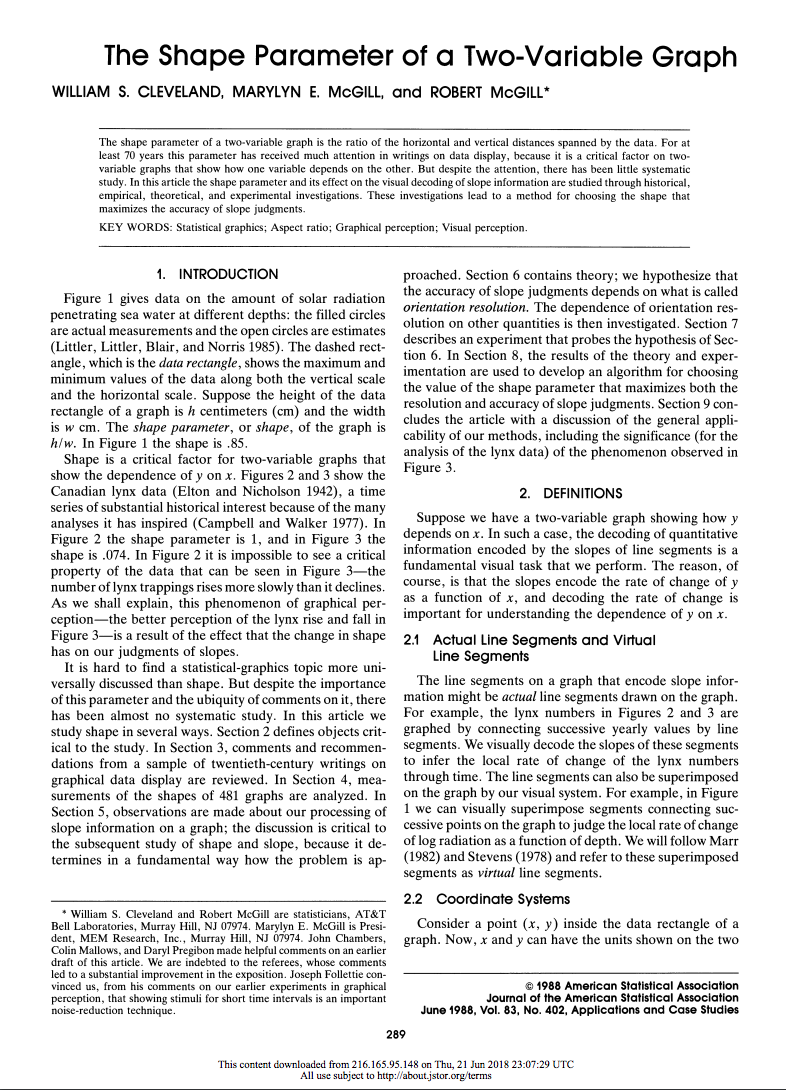
Cleveland, McGill & McGill introduced it in this 1988 JASA paper (a required reading this week)
Example: Banking to 45° Comparison
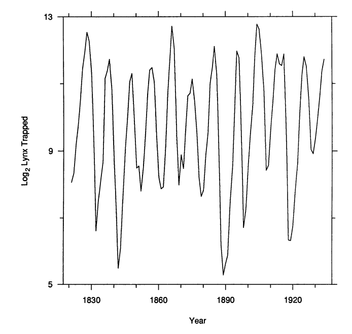
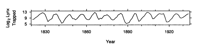
Canadian lynx trappings: a square frame (left) vs. banked to 45° (right). Which shows the shape of each cycle?
Same series twice (log2 lynx trapped per year, Cleveland’s classic example).
In the square frame every cycle is a near-vertical spike; you cannot judge how each cycle rises and falls.
Banked to 45°, the plot becomes very wide and short, and the shape of each cycle becomes something you can compare. The wide, short result is the point, not a layout mistake.
The paper’s first page is on the previous slide.
Best Practice
Rule of thumb : Always test different aspect ratios to see which one best conveys your message
Multiple Line Charts: Adding Categories
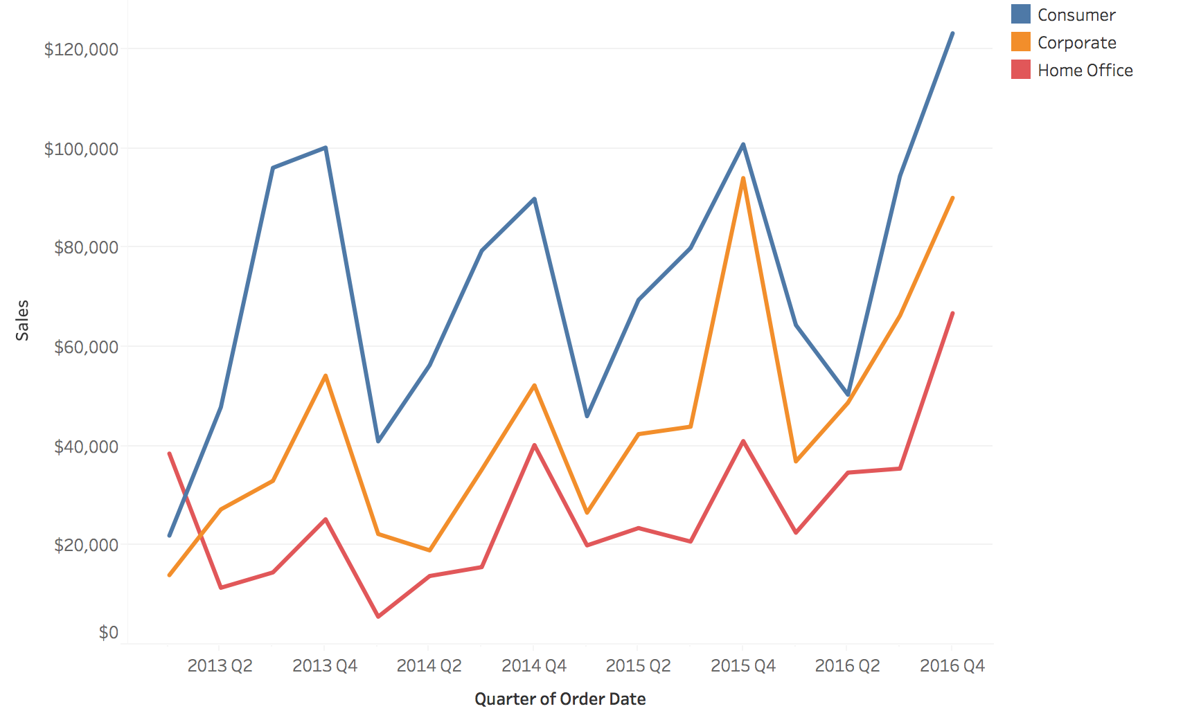
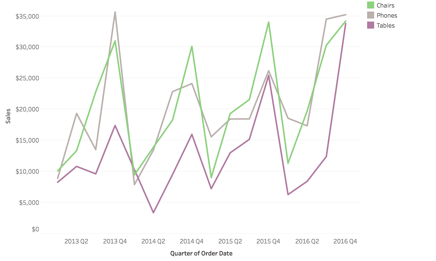
Color encodes the category: three customer segments over time.
The “Spaghetti Plot” Problem
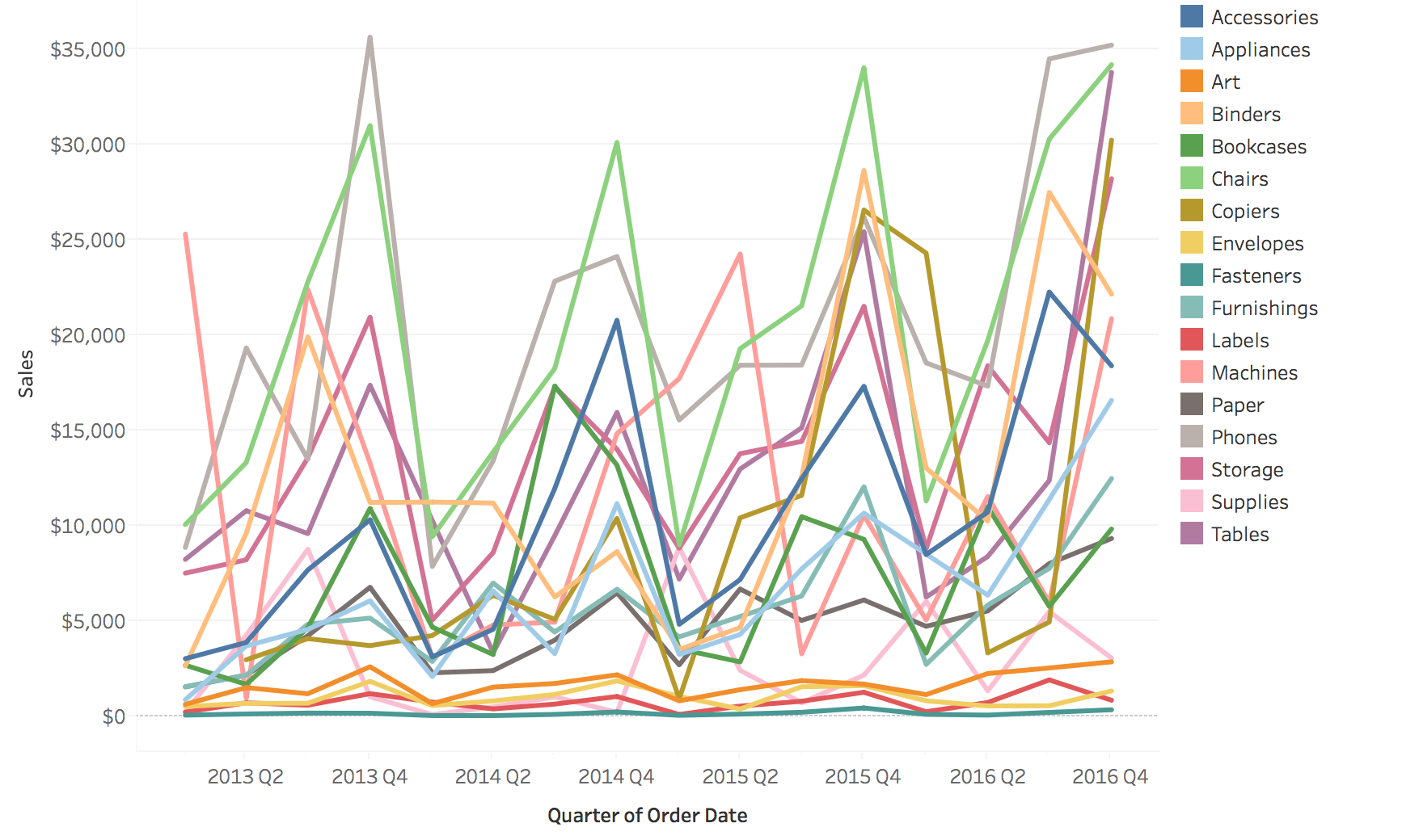
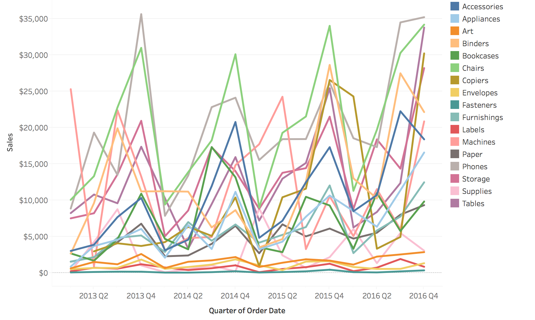
It does not scale: 17 sub-categories in one chart.
Classic problem in temporal visualization - too many lines creates visual chaos
With 50+ lines, you can’t distinguish individual series
Lines occlude each other - can’t see what’s underneath
Colors become indistinguishable - limited palette
Called “spaghetti plot” because it looks like tangled pasta!
Ask students: “Have you seen plots like this? What questions CAN you answer? What can’t you answer?”
Can answer: Overall envelope, outliers, general trend
Cannot answer: Specific values for individual series, comparisons between specific pairs
This motivates the solutions on next slides: grouping, filtering, highlighting, small multiples
Real-world example: Stock market with hundreds of stocks - spaghetti plot is useless
Solutions for Multiple Lines
Possible solutions:
Grouping
Filtering/Focus
Highlighting
Comparison: Grouping, Filtering, Highlighting
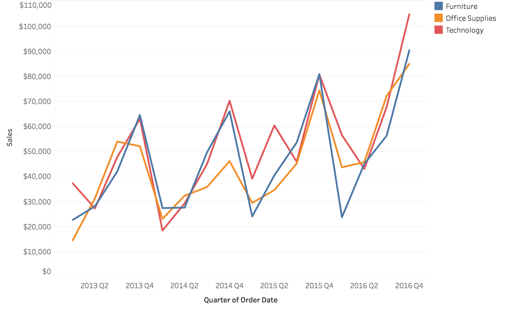
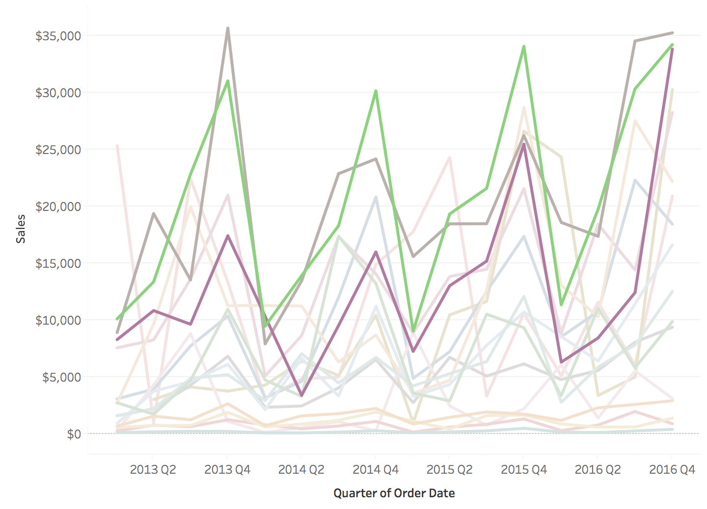
Original: 17 sub-categories
Filtering: keep 3 sub-categories
Grouping: roll up to 3 categories
Highlighting: 3 in color, the rest faded
Small Multiples
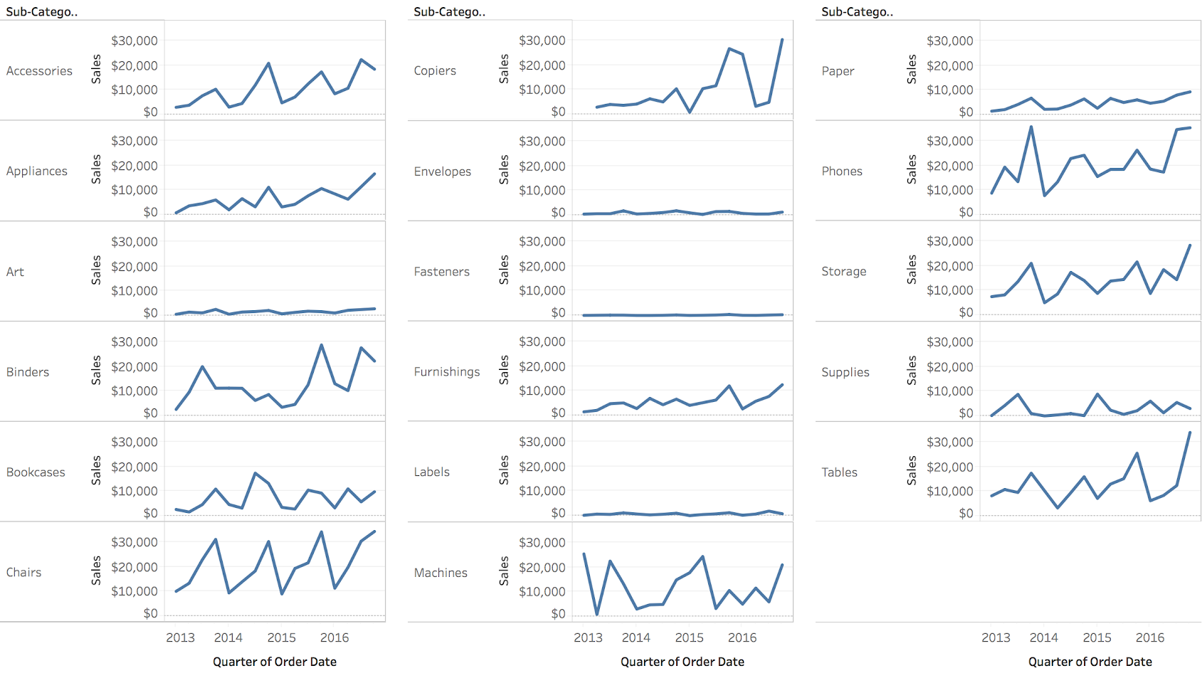
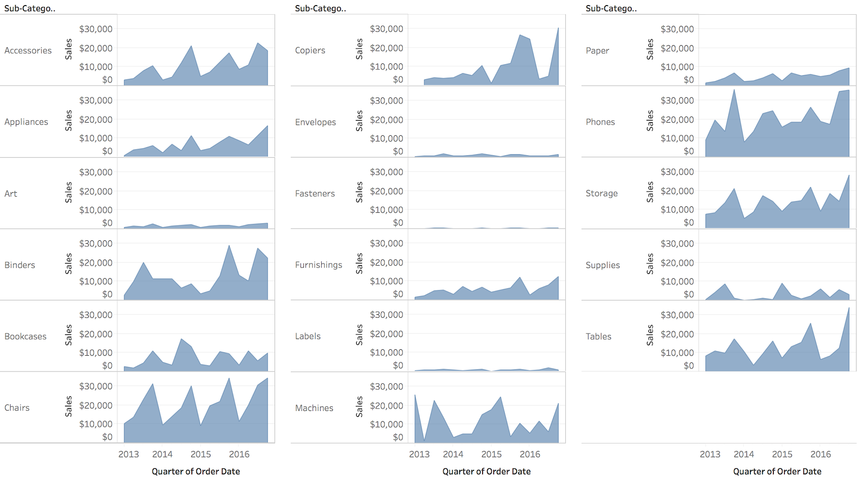
Small Multiple Line Charts and Area Charts
Small multiples = static solution to spaghetti plots
But note: Filtering and Highlighting are often INTERACTIVE techniques
This leads us to the next major topic: Interaction
Transition : “We’ve seen static solutions - but in practice, filtering and highlighting are interactive. Let’s talk about interaction techniques for temporal data…”
Example: Small Multiple Line Charts
One panel per sub-category on a shared y-axis: each series is readable and comparable.
Example: Small Multiple Area Charts
The same panels as areas: filled area emphasizes magnitude.
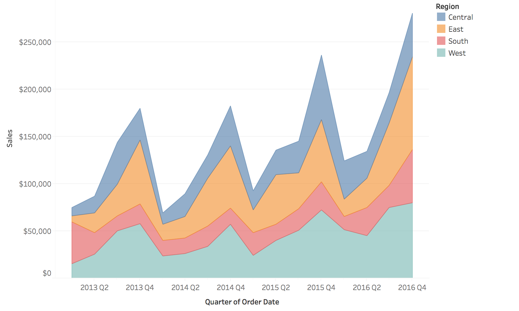
Stacked Area Charts: Total and Parts
Stacked areas show the total and how it splits across four regions.
Stacked Area Charts: Limitations
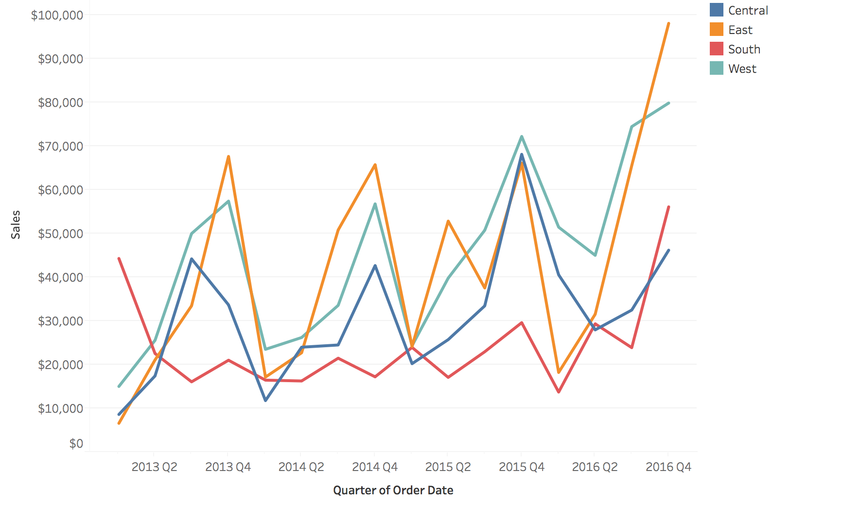
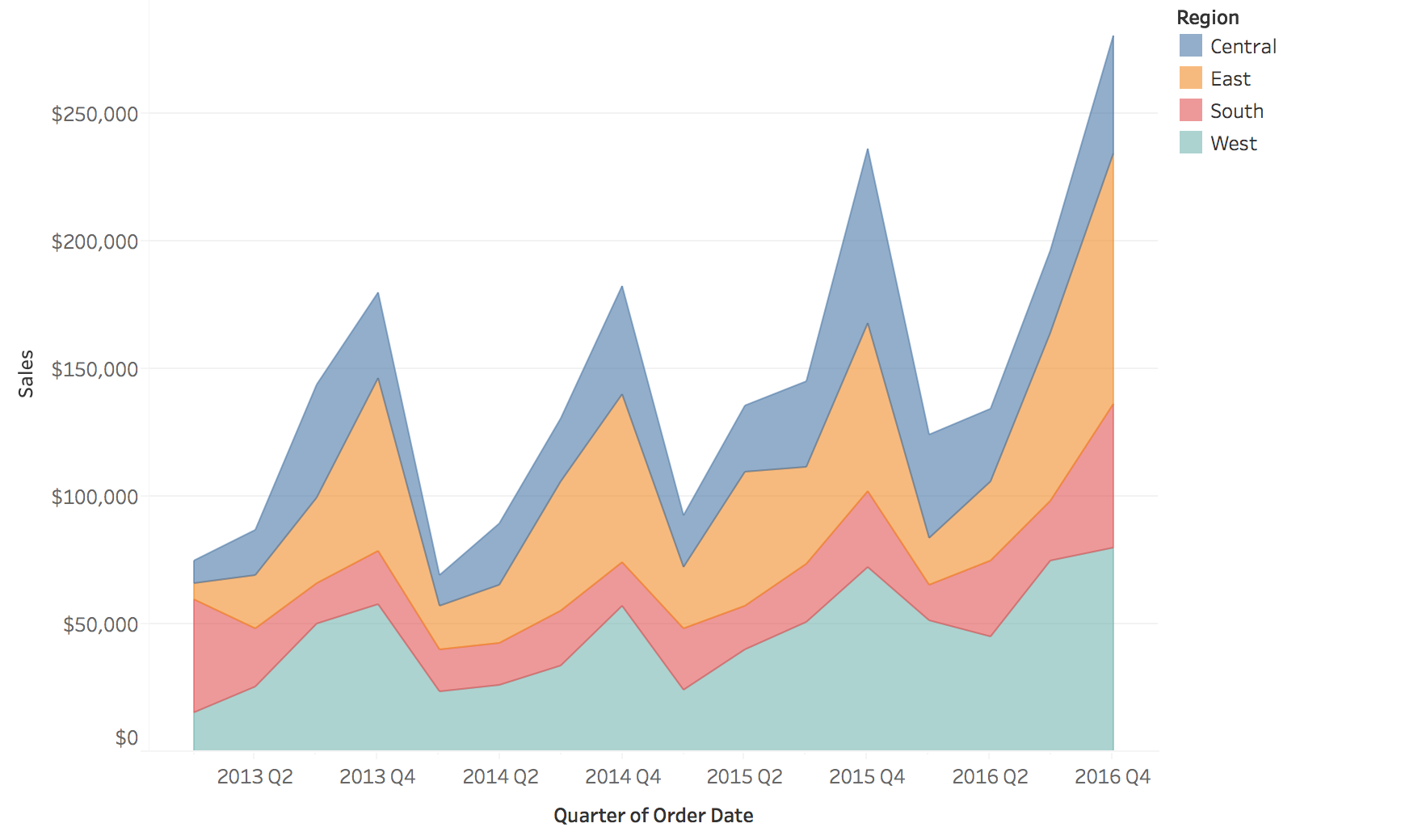
“Baseline bias”: only the bottom layer sits on a common baseline.
The same four regions as lines (left) and stacked (right). Try reading East’s trend on the right.
Problem: temporal trends for upper layers are hard to interpret because they don’t share a common baseline
In this figure East is orange, West (teal) is the bottom layer
IMPORTANT PERCEPTUAL LIMITATION - students often misuse stacked area chartsThe bottom layer (touching x-axis) is easy to read - it has a stable baseline
But upper layers “float” on changing baselines - very hard to judge their values or trends
INTERACTIVE DEMO : Point to an upper layer (e.g., green category) and ask:
“Did this category increase or decrease between these two time points?”
“Can anyone tell me the actual value for this category in Q3?”
Students will struggle - this proves the baseline bias!
Then show: Only the bottom layer can be read accurately
The total height is easy to read, but individual layer trends are ambiguous
Example: If bottom layer increases sharply, upper layers appear to go up even if their actual values are flat
When to use: When you care about total AND composition, and bottom layer is most important
When NOT to use: When you need to compare trends across all categories
Better alternatives: Small multiples (separate charts), normalized stacked (next slide), or just don’t stack
Real example: COVID dashboards with stacked areas - very misleading for comparing different variants
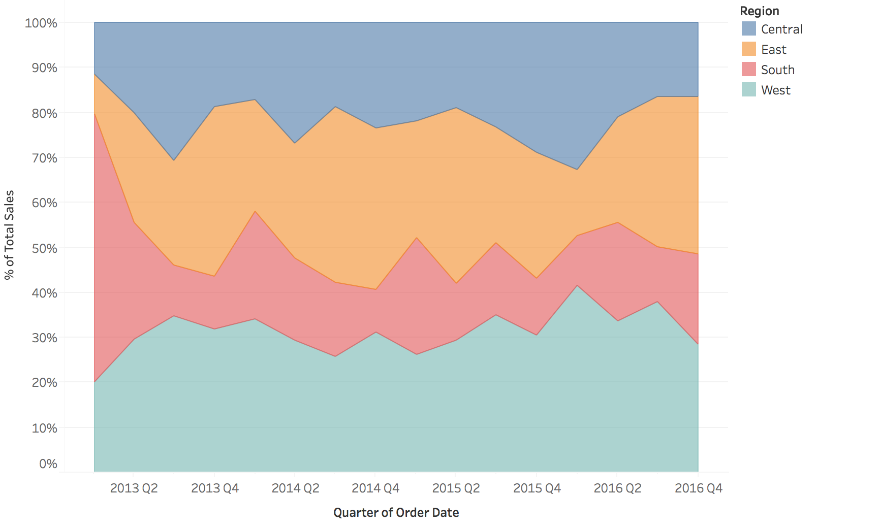
Normalized Stacked Area Charts
Normalized to 100%: composition only, the total is gone.
Interaction Techniques
Critical for exploring temporal data
Why Interaction Matters for Temporal Data
Challenge : Time series data is often too large or complex to understand in a single static view
Solution : Interactive techniques allow users to:
Navigate through time (zoom, pan)
Focus on specific patterns or events
Link multiple views for comparison
Dynamically adjust aggregation levels
Zoom and Pan
Purpose : Navigate dense sequential time series
Semantic Zoom
Change level of detail
Hourly → Daily → Monthly
Preserve context
Geometric Zoom
Magnify visual space
See more detail
Focus + context techniques
Example : Stock chart with overview + detail panes
Two fundamentally different types of zoom - students often confuse these!
LINK BACK : “Remember our Aggregation Trade-offs slide? Semantic zoom is interactive aggregation!”Semantic Zoom = change aggregation level (connect back to earlier aggregation slide)
Zoom out: Hourly → Daily (aggregate 24 hours into 1 point)
Zoom in: Daily → Hourly (show finer resolution)
Data actually changes - different level of detail
This lets you explore different aggregation levels interactively rather than committing to one upfrontExample: Google Maps showing cities vs streets vs buildings
Geometric Zoom = magnify the view (like a magnifying glass)
Same data points, just bigger
Doesn’t change aggregation, just visual scale
Example: Zoom into a region of a line chart to see fluctuations better
Best practice: Combine both - overview + detail where overview provides context
Example to show: Stock charts with small overview at bottom + zoomed detail above
Interaction: Brushing in overview selects region shown in detail
Filtering and Brushing
Filtering : Show/hide data based on criteria
Time range selection
Category filtering (e.g., show only certain products)
Threshold filtering (e.g., values > X)
Brushing : Select data in one view, highlight in others
Temporal brushing : Select time range, see corresponding eventsLinked views : Brush on map → highlight in timeline
Brushing & Linking Example
View 1 : Geographic map
User brushes (selects) a region
View 2 : Time series
Corresponding temporal data highlights automatically
Power : Discover spatio-temporal patterns (e.g., “Sales peak in Region A during Q4”)
LIVE DEMO OPPORTUNITY : If you have a prepared D3 example, Tableau dashboard, or Observable notebook, SHOW THIS LIVE
Static images can’t convey the interactivity
Seeing the linking happen in real-time is 100x more impactful
Even a simple example (brush a time range, see map update) will make this memorable
If no live demo available: At minimum, verbally walk through the interaction
“Imagine I click and drag on the map to select this region…”
“…instantly, the time series highlights just those data points”
“Now I can see: this region has a spike every December”
This is the payoff of brushing & linking - cross-view pattern discovery
Dynamic Aggregation
Interactive granularity control
Users adjust time resolution on-the-fly:
Slider: “Show me data aggregated by: Hour / Day / Week / Month”
Drill-down: Click on a month → see daily breakdown
Roll-up: Aggregate noisy hourly data to daily averages
Advanced : Time-series bagging, dynamic binning for very long series
Time Warping and Distortion
Fisheye/distortion :
Focus region shows detail
Context regions compressed
Maintains overview while examining specifics
Time-warping :
Align periodic patterns despite phase shifts
Dynamic time warping (DTW) for comparing similar patterns
Useful for comparing multiple time series with lag
Best Practices for Interaction Design
Provide overview first : Show full temporal extentProgressive disclosure : Start simple, reveal detail on demandMaintain context : Always show where you are in timeLink multiple views : Connect temporal, spatial, and categorical viewsSmooth transitions : Animate changes to maintain mental modelDirect manipulation : Let users interact with the visualization itself
Event Data Visualization
Visualizing discrete events and durations
Types of Event Data
Timestamp + Event Properties
Incidents
Activity Logs
Messages (Emails, Chats, etc.)
Example: Dot Plot for Events
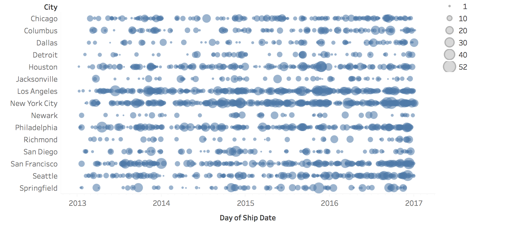
Rows = cities, x = ship date; dot size encodes a count (legend 1-52).
Example: Proportional Symbols plus Color
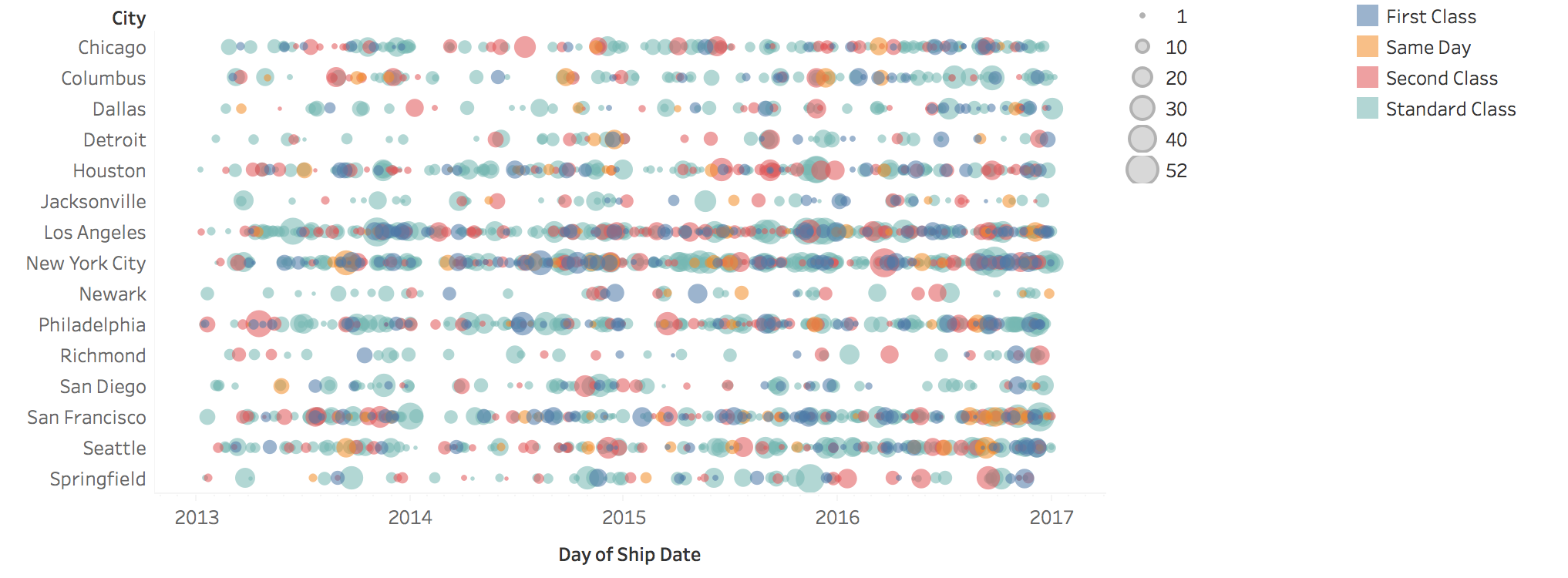
The same dots colored by ship mode: size and color carry two event attributes.
Events with Duration
How do you visualize events that have duration?
Gantt Charts
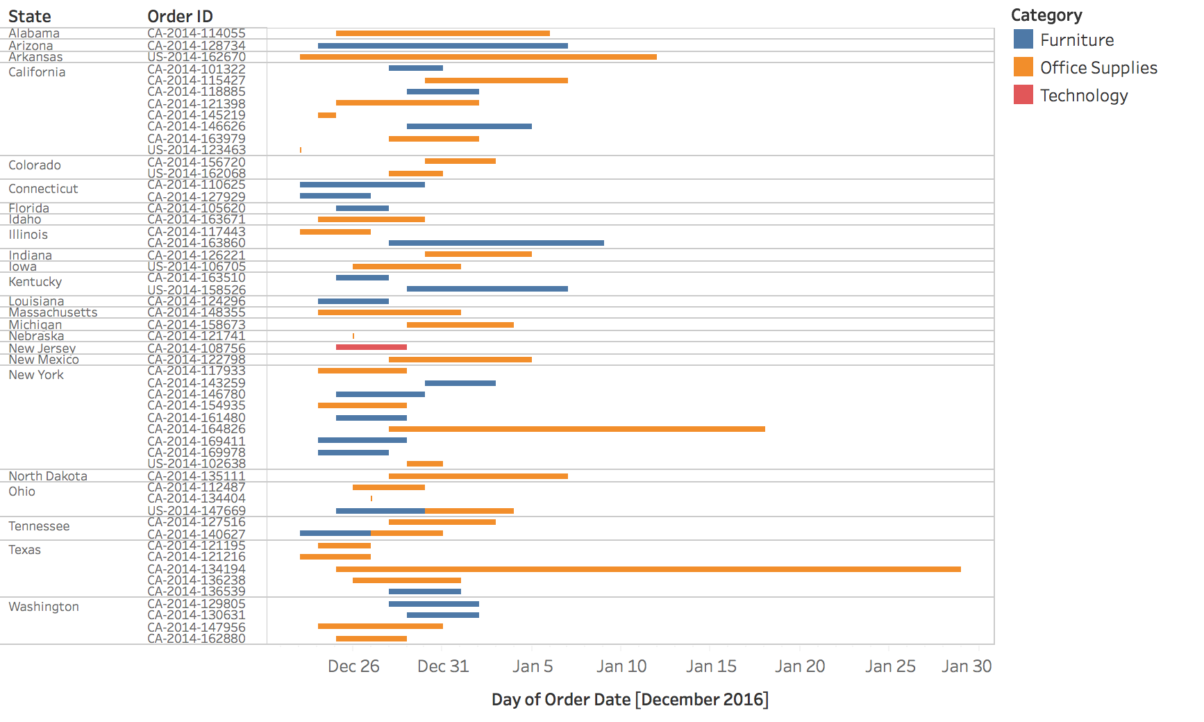
Horizontal bars show each event’s start, duration, and end.
CONNECT BACK TO EVENT DATA : “Remember our Event Data definition? Events with duration? Gantt charts are THE classic visualization for this.”Origin story : Named after Henry Gantt (1910s) - originally invented for project management
Shows tasks, dependencies, timelines
Still dominates project management software (MS Project, Asana, Jira, etc.)
Modern applications have expanded far beyond projects:
Server/system activity monitoring (next slides)
Resource allocation (people, machines, rooms)
Manufacturing schedules
Any scenario with concurrent activities over time
Key visual features:
Time on x-axis
Tasks/resources on y-axis
Bars show start, duration, end
Can show dependencies with arrows
Example: Gantt Chart
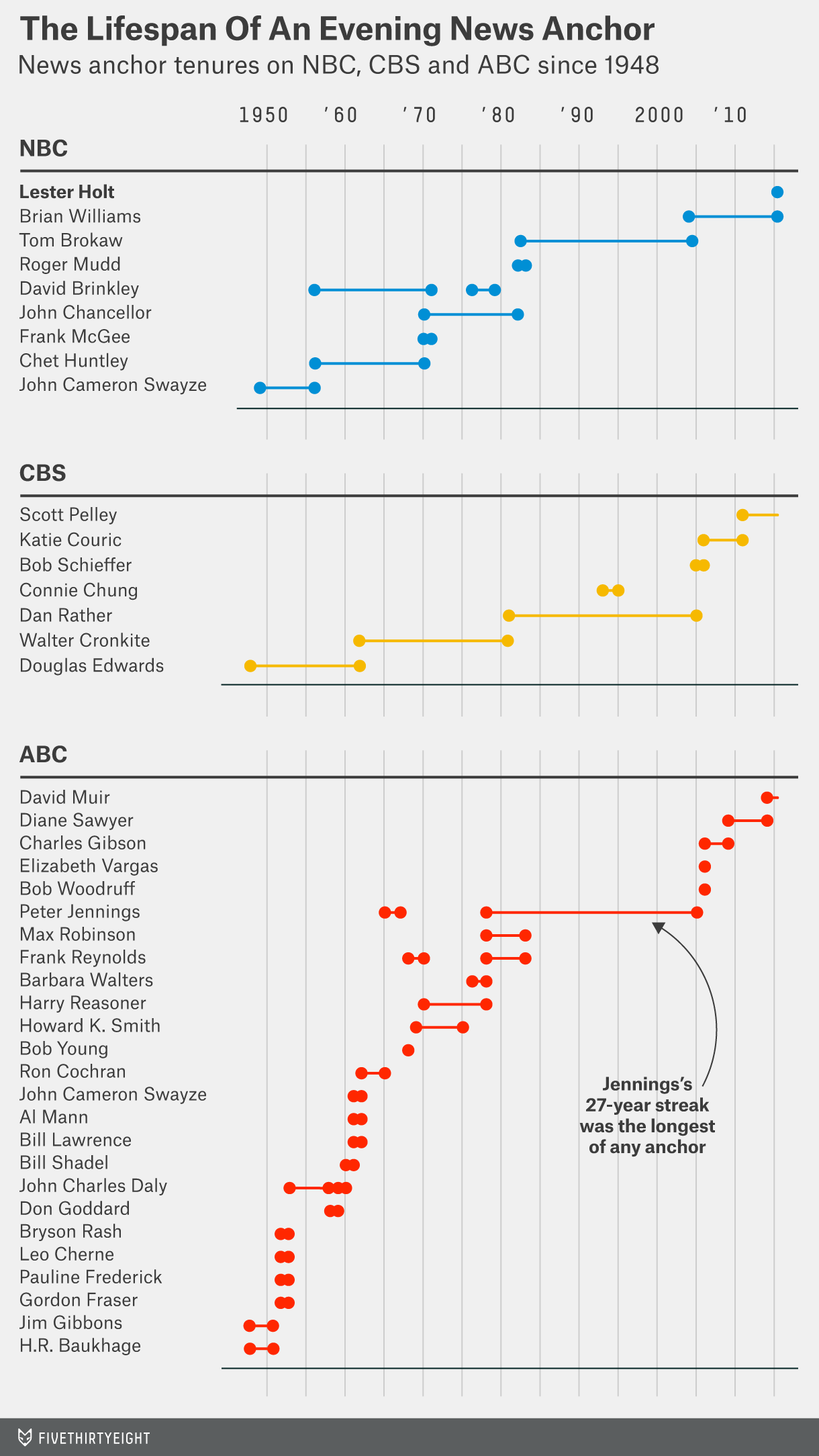
The lifespan of an evening news anchor
One row per anchor, grouped by network (NBC, CBS, ABC), since 1948
A line from start to end shows each tenure
The annotation calls out the longest run: Jennings, 27 years
Example: System Activity Monitoring
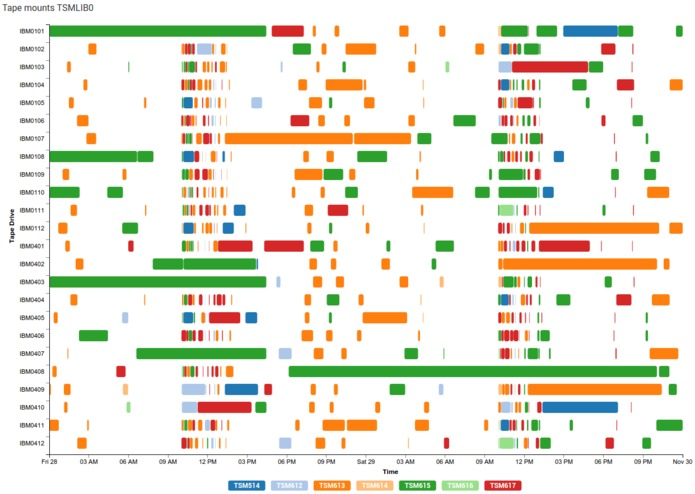
Tape mounts per drive over a day and a half: concurrent activity at a glance.
Periodic Patterns
Calendars, radial layouts, and spirals
OPTIONAL SECTION - If running short on time, you can skip spirals and cover calendars quickly (10 min) - Calendars are most practical for students - Radial layout warnings are important (5 min) - Spirals are interesting but not essential
Understanding Periodicity
Often the focus is on investigating and presenting periodical patterns:
Yearly, seasonal, monthly
Weekly, daily, hourly
Alternative Approaches
One line per year across the week: what else could show this periodic pattern?
Calendar-Based Visualizations
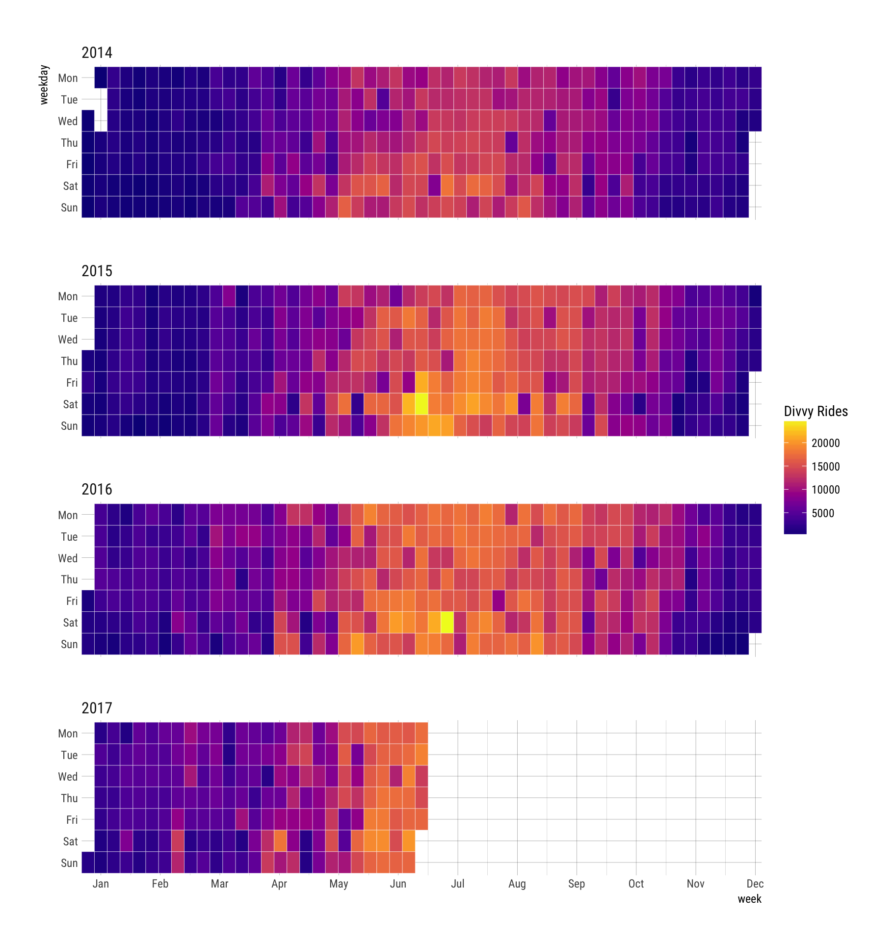
Key difference from heat maps : time is laid out by day-of-week and month
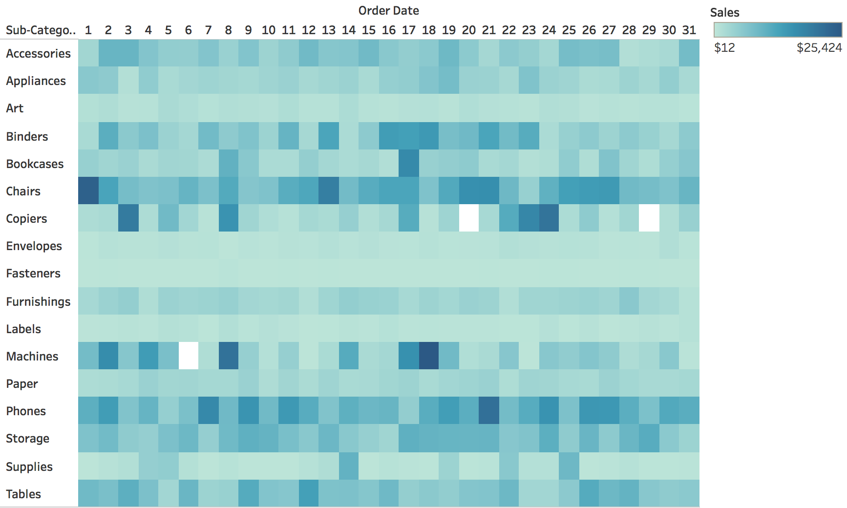
Heat maps : linear time progressionCalendar views : explicit cyclic layout (7-day weeks, 12 months)Better for weekly and seasonal patterns
Here: Divvy bike-share rides per day, 2014-2017
Calendar views leverage our familiarity with calendar structure
Key insight: Days of the week align vertically - easy to spot weekly patterns
Example: Website traffic calendar - weekend days align vertically, immediately see weekend dip
Difference from heat maps:
Heat maps: continuous time, arbitrary row breaks
Calendars: structured by weeks/months, meaningful breaks
When to use calendars:
Data with strong weekly patterns (work/weekend differences)
Data people think about in calendar terms (appointments, events, habits)
Limitations:
Only works for day-level or finer granularity
Months have different lengths - creates visual gaps
Not good for long time spans (multiple years gets unwieldy)
Real examples: GitHub contribution calendar, fitness tracking apps, habit trackers
Ask: “What apps use calendar views? Why does it work for them?”
Calendar Variations
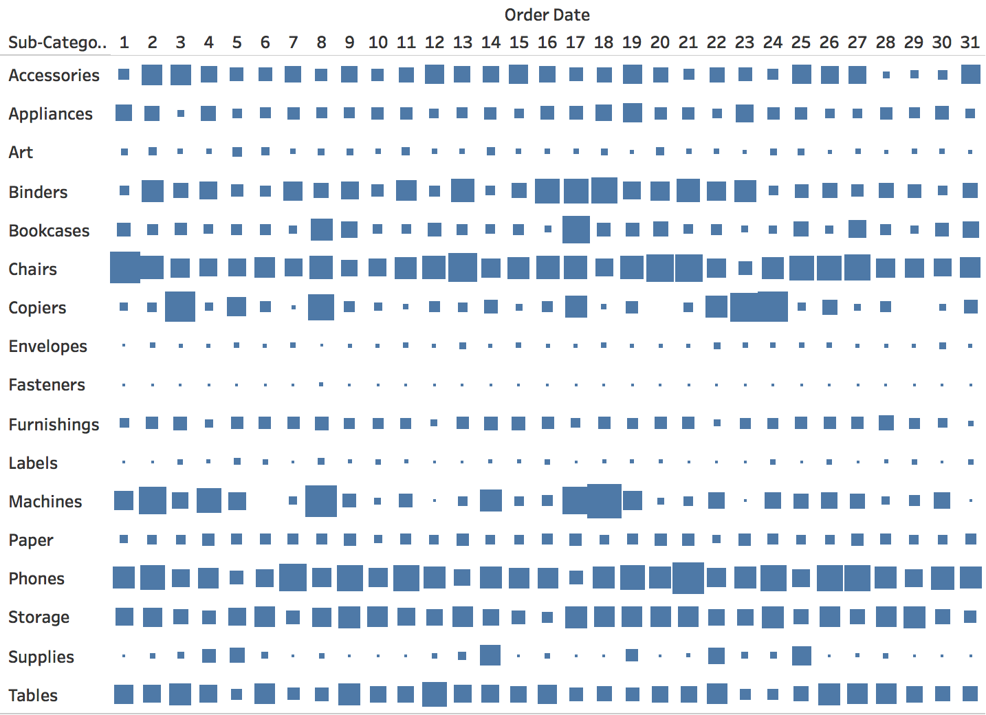
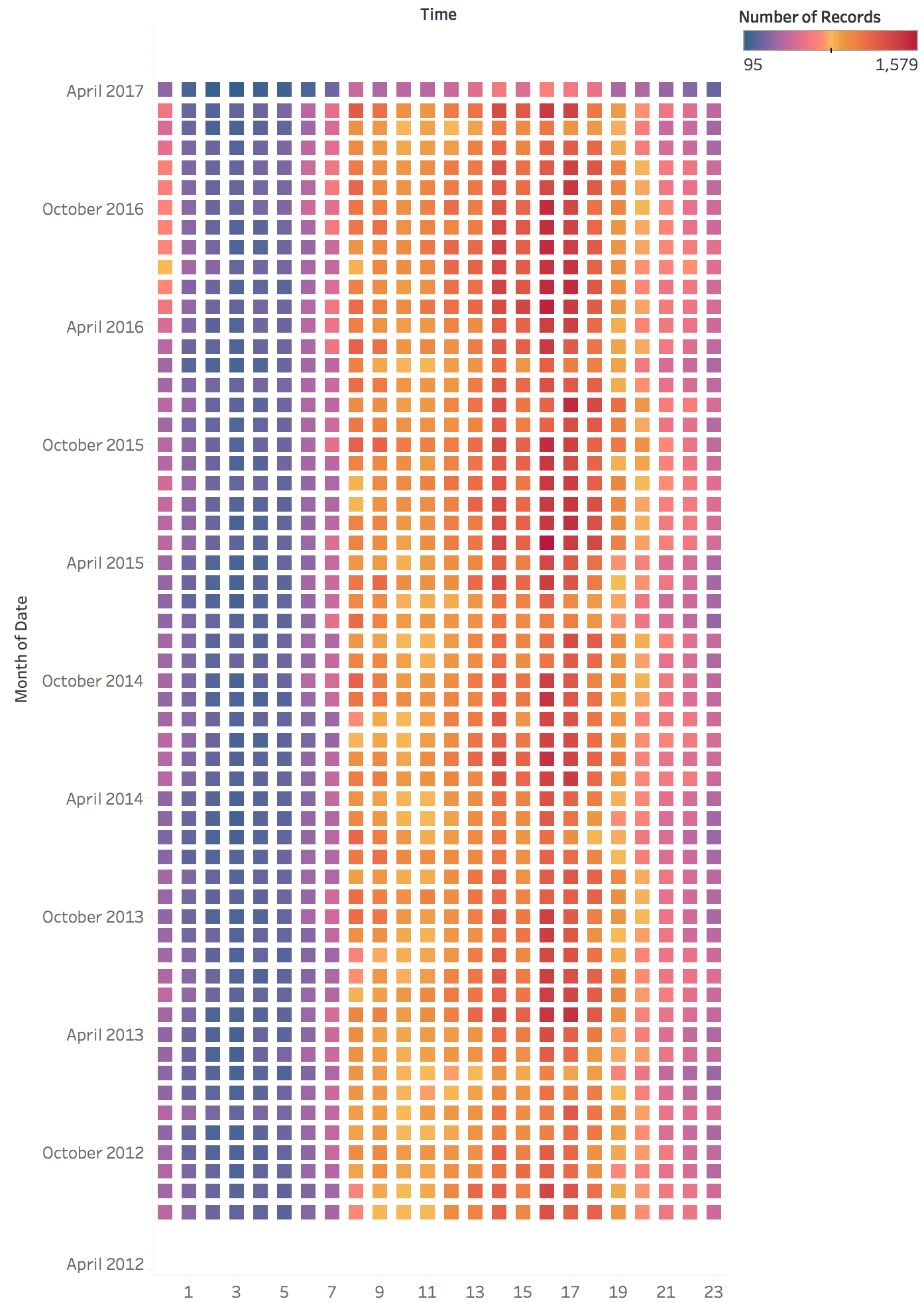
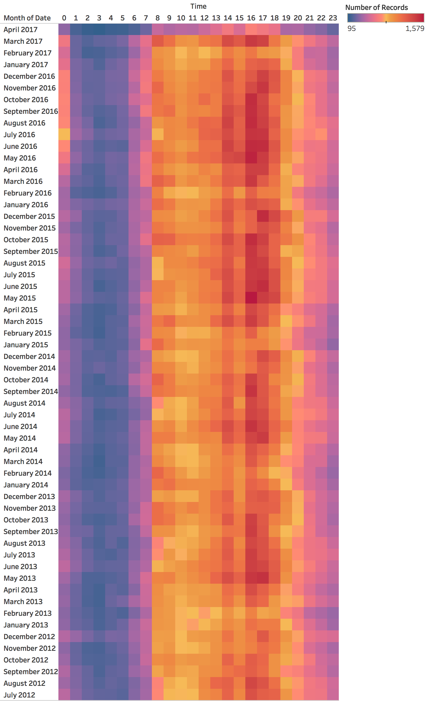
Month × hour of day, two ways: a grid of marks (left) and a continuous heat map (right).
Radial Layouts for Periodic Data
Periodic phenomena are cyclical. Radial layouts can reduce temporal discontinuities
Spiral Plots
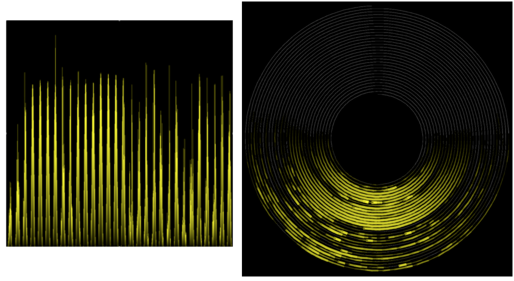
Key insight : spirals show cycles and progression at the same time
Cycles : the same phase of each period sits at the same angleProgression : each turn moves outward in timeWeber et al.: the same periodic series as a line (left) and a spiral (right)
The brilliance of spirals : They encode TWO temporal structures at once
Cyclic structure : Each complete rotation = one cycle (year, month, day)Sequential structure : As you spiral outward = progression through time Temperature example (next slide):
Angle = month of year (seasonal cycle)
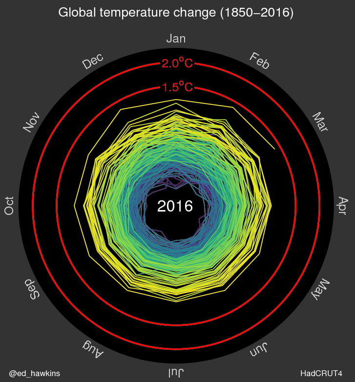
Radius = temperature anomaly, NOT year; color = year (purple 1850s to yellow 2010s)
So Hawkins’ spiral is a radial line chart with one loop per year rather than a Weber spiral: outward = warmer
The climate spiral makes the warming vivid: later (yellow) loops sit further out
Trade-off: Harder to read precise values (radial layout limitations)
Use when: The dual encoding (cycle + trend) is more important than precision
Spiral Example: Temperature Data
Angle : month of the yearRadius : temperature anomaly vs. 1850-1900 (red rings at 1.5 °C and 2.0 °C)Color : year, purple (1850) to yellow (2016)Later loops sit further out: warming
Climate Spiral Visualization
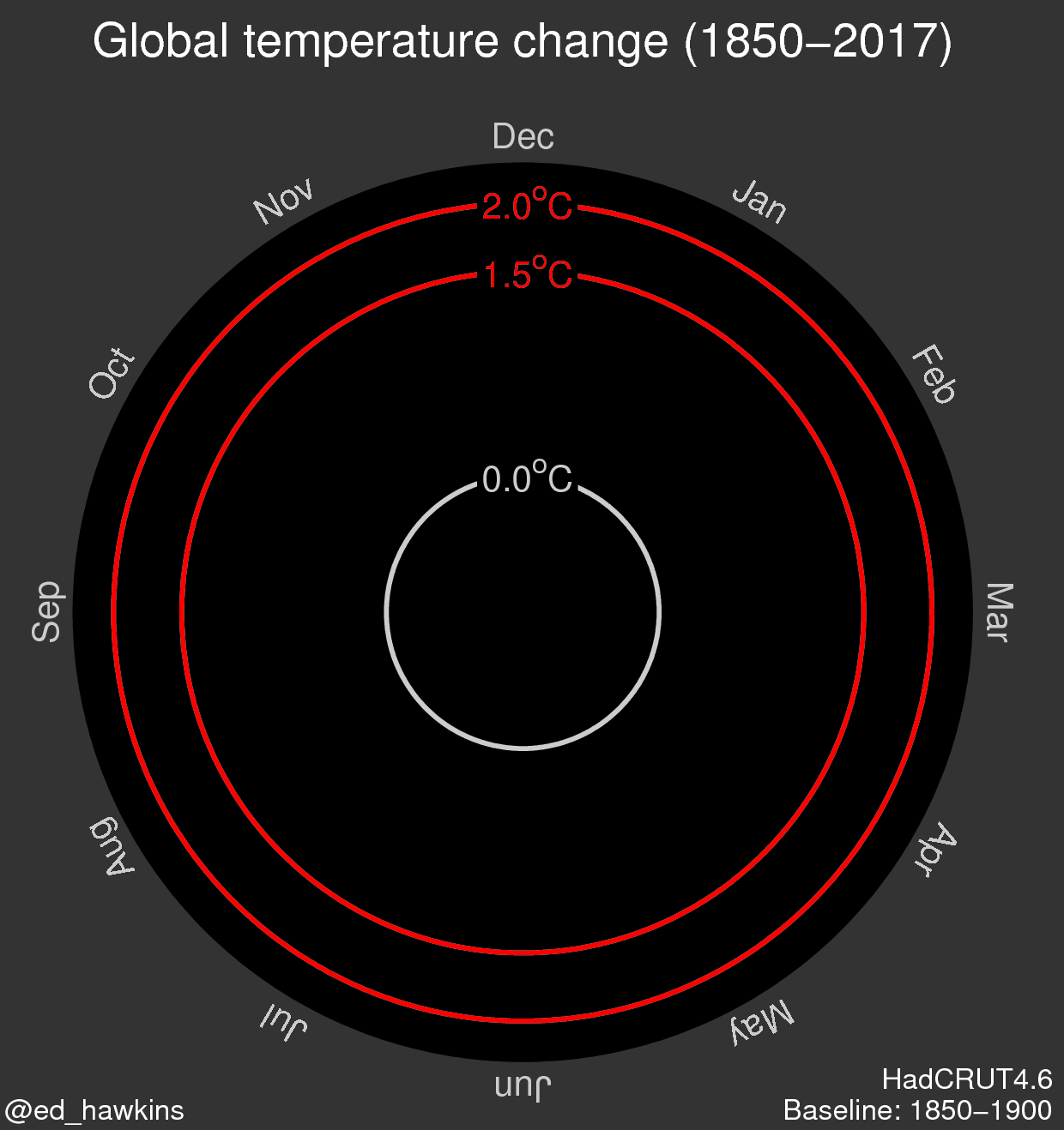
The animated version draws one loop per year, month by month, from 1850 to 2017
This still is its first frame, before any data is drawn
Play the animation to watch the loops push toward the 1.5 °C ring
Caution: Radial Layout Limitations
Use circular layouts with care!
Research finding : Humans are significantly slower and less accurate at judging radial distances and angles compared to linear position
Comparing values radially is harder than in Cartesian space - use only when cyclical nature is essential
CRITICAL WARNING - radial layouts look cool but are perceptually problematicResearch shows 2-3x slower and less accurate judgments in radial vs linear layouts
Why are they harder?
Angles are harder to judge than horizontal/vertical distances
Outer rings have more space than inner rings (same value, different visual area)
Hard to compare values at different angles
When ARE they appropriate? When emphasizing cyclical nature is more important than precise reading
Example: 24-hour clock pattern - circular makes sense conceptually
Example: Climate spiral - the spiraling metaphor communicates urgency
But for most analytical tasks: stick to linear layouts!
Ask: “When have you seen radial visualizations in the wild? Were they effective?”
Common misuse: Corporate dashboards with radial charts just because they look fancy
Comparison: Linear vs Radial
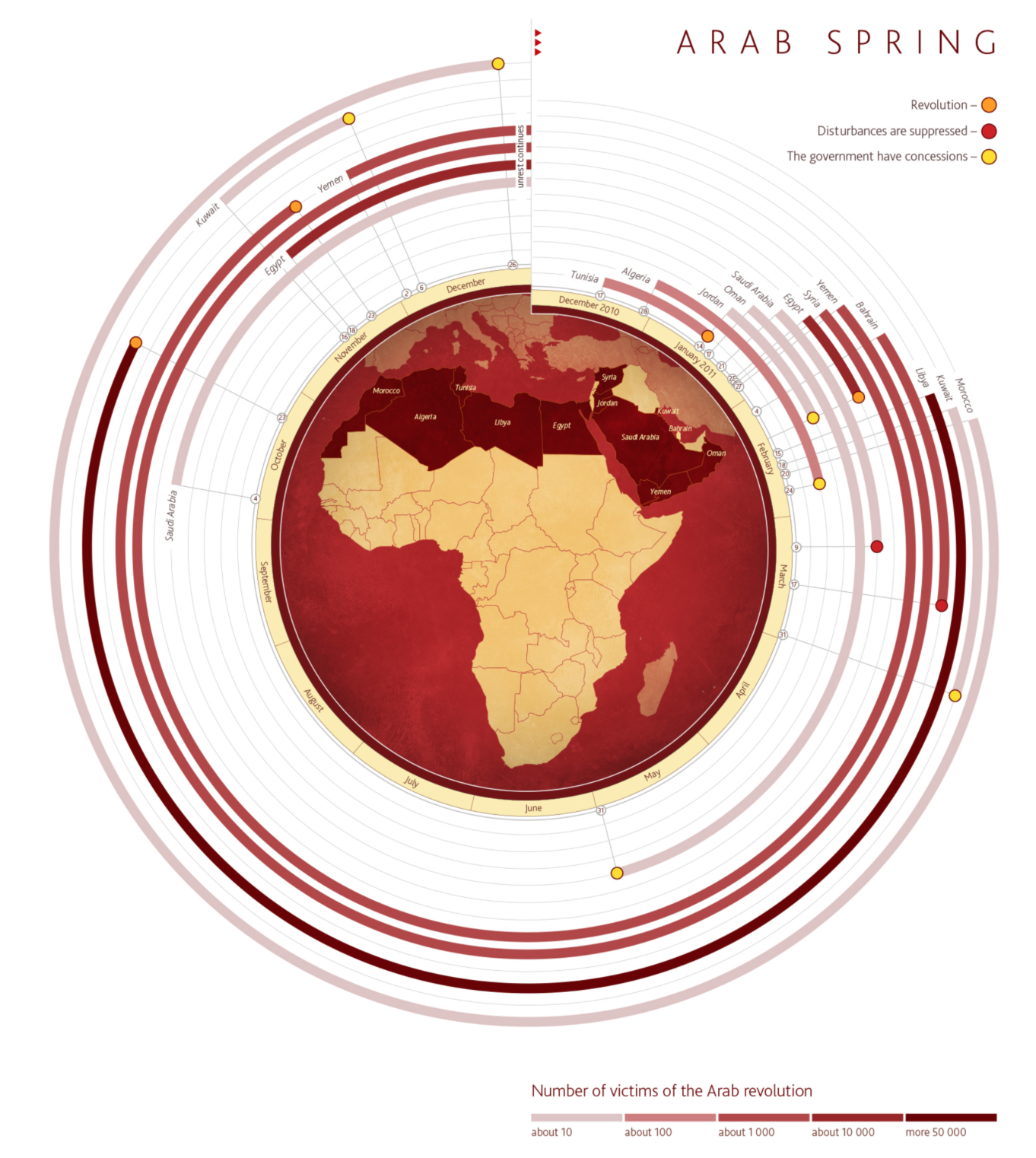
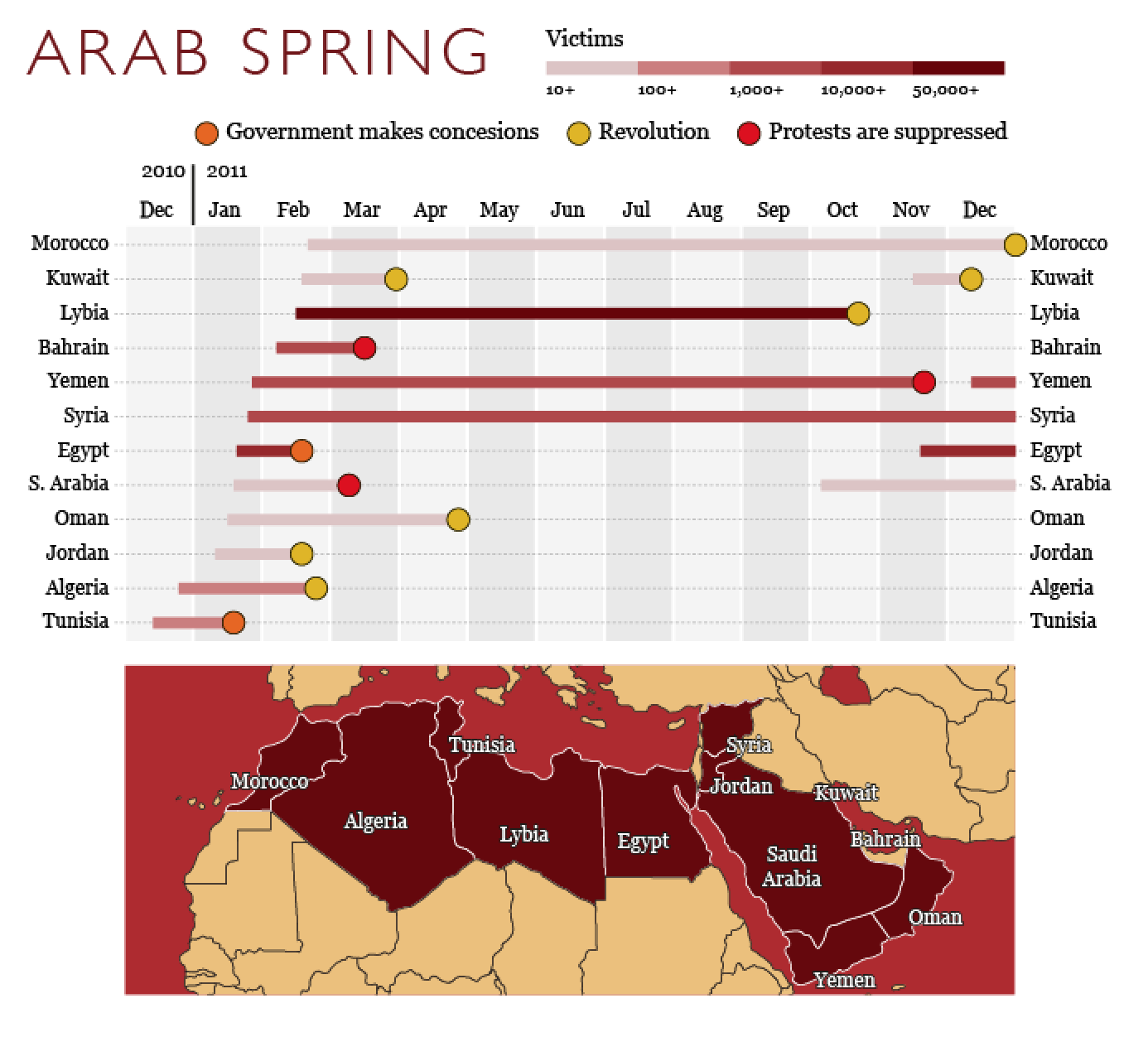
Arab Spring timeline, radial (left) vs. linear (right): which makes durations easier to compare?
Scalable Visualizations
Horizon charts and sparklines for dense temporal data
ADVANCED/OPTIONAL SECTION - This can be assigned as reading if short on time - Horizon charts are complex and need 15 min to walk through properly - Sparklines are quick (5 min) and useful, show if you can - If pressed for time: Show the horizon chart concept but assign the step-by-step as reading - Students don’t NEED to build horizon charts, but should know they exist
Horizon Charts
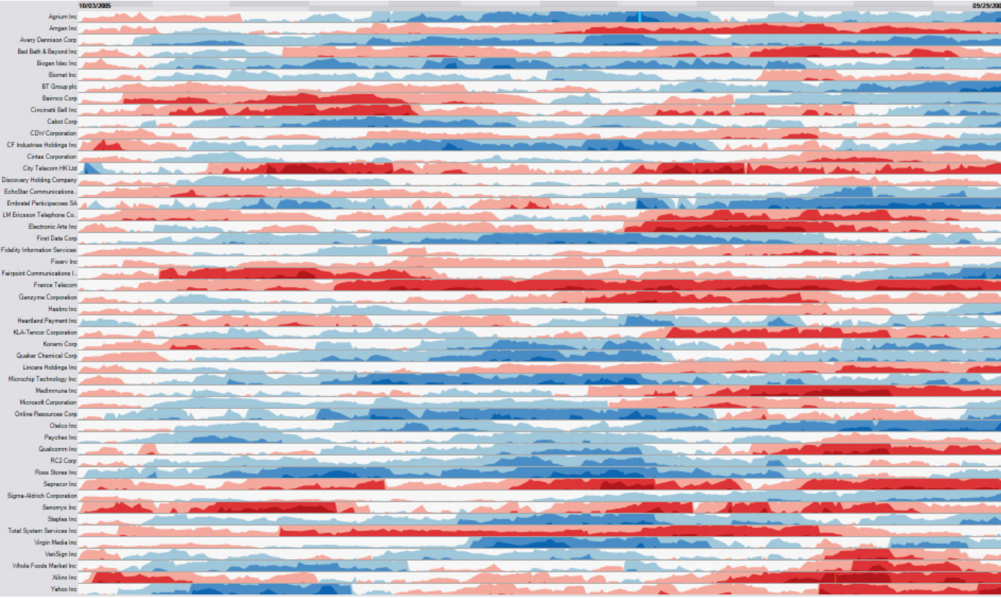
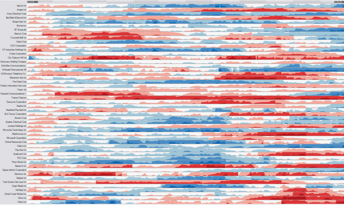
Maximum density in minimal height: dozens of time series compared at once.
Advanced technique - horizon charts solve a specific problem: showing MANY time series compactlyProblem: Line charts need vertical space - can only show ~10 series before running out of screen space
Horizon charts compress vertical space by 2-4x while maintaining readability
Used in: Server monitoring dashboards, financial data with hundreds of stocks, climate data arrays
Key innovation: Trade vertical space for color intensity
CRITICAL : This looks like “magic” unless you understand the constructionNext slides walk through step-by-step : This is NOT optional - you MUST show the construction process
Without understanding HOW it’s built, students will just see a confusing colored chart
The 4-step process (area → bands → flip → collapse) demystifies it
Heer et al.’s paper/video has excellent animations of this - reference them
Takes practice to read - not intuitive at first glance
Heer et al.’s CHI paper showed horizon charts can be as accurate as line charts but in 1/4 the space
Real-world example: Cubism.js library for real-time dashboards
When to use: When you have >20 time series and need to see them all simultaneously
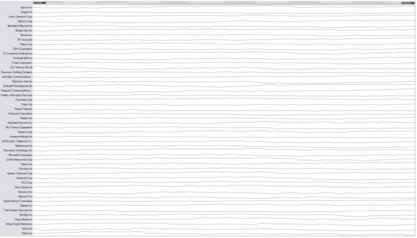
Why Not Line Charts? Same Series, Same Height
The same series as plain line charts at this height: almost flat, nothing to read.
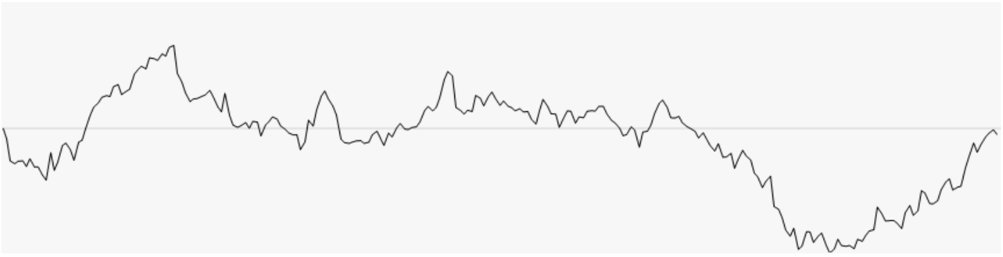
How Horizon Charts Work: Step 1
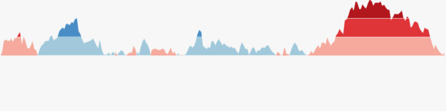
Start with a standard area chart.
SLOW DOWN : Take your time with these construction slidesStep 1 is familiar - just a normal area chart
“This is what we know - a regular area chart. Now watch what happens…”
Make sure students understand this baseline before moving forward
Step 2: Discretizing into Bands
Divide values into equal-height bands (e.g., 0-1, 1-2, 2-3).
Key transformation #1 : Chop the area into horizontal slices“We’re dividing the chart into bands of equal height”
Point to each band: “0-1 gets one color, 1-2 gets another, 2-3 gets a darker shade”
This is like creating a color scale for elevation on a topographic map
Make sure students see: Same data, just segmented into layers
Step 3: Flipping Negative Values
Mirror negative values above the baseline, told apart by hue.
Key transformation #2 : Handle negative values“Notice negative values? We flip them UP above the baseline”
Use different color (or saturation) to distinguish positive from negative
In this figure blue = positive, red = negative
Why flip? Because next step collapses everything - we need both directions in same vertical space
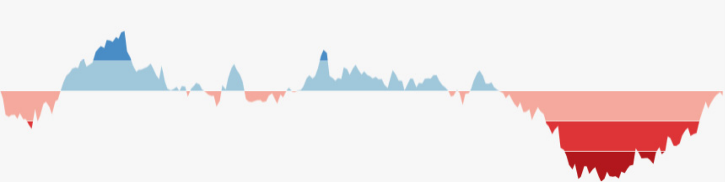
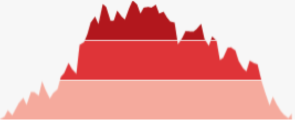
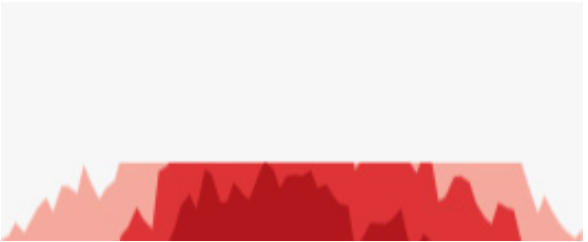
Step 4: Collapsing Bands
Overlay the bands in one strip (left to right): darker = larger magnitude.
THE MAGIC STEP : Now we collapse all the bands into the same vertical space“All those layers we created? We stack them on top of each other”
This is the key insight : Height → Color intensity
Band 1 (0-1): Light color
Band 2 (1-2): Medium color (stacked on top, shows darker)
Band 3 (2-3): Dark color (all three stacked)
The result: Same temporal patterns, but 1/3 the height
“Look at the before and after - same pattern, compressed vertically”
This is why color intensity = magnitude in horizon charts
Final Result: Horizon Chart
A compact view that keeps temporal patterns in minimal height.
Recap the transformation : “We went from area chart → banded → flipped → collapsed”Now students should understand WHY darker colors = higher values
“Without understanding the construction, this just looks like random colored bands”
“But now you know: it’s a compressed area chart where height became color intensity”
Practical reading tip: Darker/more saturated = higher magnitude
Point out: You can still see the temporal patterns (peaks and valleys), just compressed
Reference Heer’s work : “The original CHI paper and video show this animation - highly recommended”
Sparklines
“Small, intense, word-sized graphics with typographic resolution. Sparklines can be placed anywhere that words or numbers can be: in sentences, maps, graphics, tables.”
— Edward Tufte
Edward Tufte’s concept - minimal, inline visualizationsPhilosophy: Data should be integrated into text, not separated
Key characteristics:
No axes, no labels, no gridlines - just the trend
Fits inline with text (same height as text line)
Shows pattern at a glance, not precise values
“Data-intense, design-simple, word-sized”
When to use: Tables, dashboards, reports where you want to show trend alongside numbers
Example: Stock table showing current price + sparkline of last 30 days
Not for: Detailed analysis, precise reading, standalone charts
Implementation: Easy in modern tools (Excel, Tableau, D3, etc.)
Ask students: “Where have you seen sparklines? What made them effective?”
Common examples: Google Finance, Twitter analytics, GitHub contribution graphs
Sparklines in Context
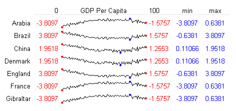
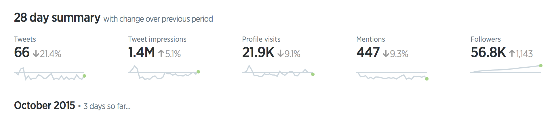
In a table (top) and a dashboard summary (bottom): the data becomes part of the text.
Sparkline Examples
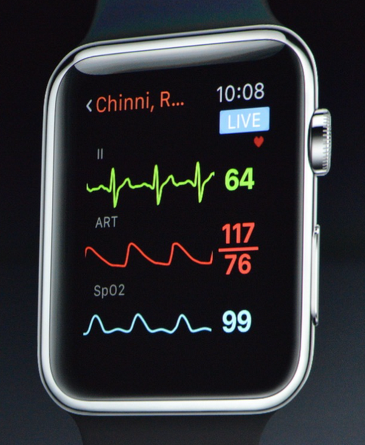
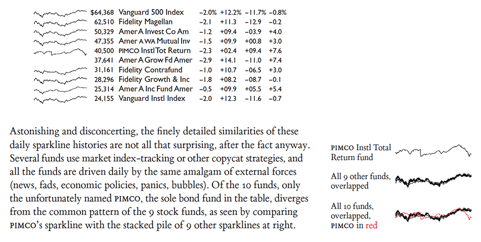
On a watch face (left) and in Tufte’s mutual-fund table (right).