# Introduction Based on materials by Enrico Bertini NYU Tandon School of Engineering ::: notes **LECTURE TIMING GUIDANCE (150 min total)** **Part 1: Networks (70 min)** - Network fundamentals (10 min) - Force-directed layouts (20 min) - Fixed layouts & edge bundling (15 min) - Matrices & clutter reduction (15 min) - Wrap-up & quiz (10 min) **Part 2: Trees (70 min)** - Tree fundamentals (10 min) - Node-link trees & examples (15 min) - Dendrograms (10 min) - Decision trees (10 min) - Treemaps (20 min) - Sunburst/Icicle plots (5 min) **Wrap-up (10 min)** - Summary & programming assignments ::: --- # Part 1: Networks Objects, relationships, and visualization approaches --- ## Network Data Fundamentals ::: {.columns} ::: {.column width="50%"} **Network Data = Objects + Relationships + Values** - **Objects**: Nodes (people, cities, genes) - **Relationships**: Edges (friendships, routes, interactions) - **Values**: Node attributes (age, size) & edge attributes (weight, type) ::: ::: {.column width="50%"} 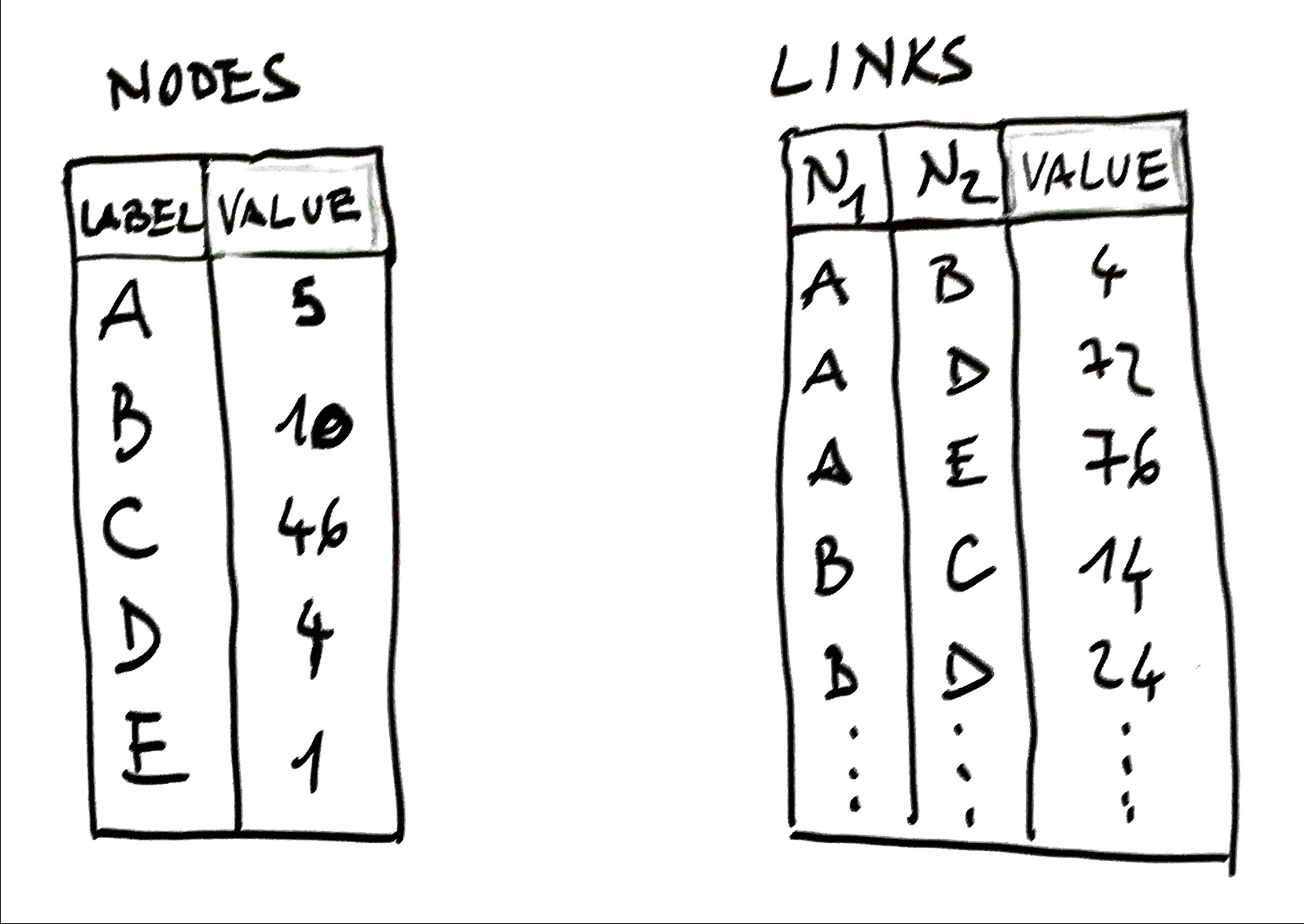 ::: ::: **Application Domains**: Social networks, biological systems, transportation, web, infrastructure ::: notes - Network data is one of the most fundamental data structures - Key distinction: We care about RELATIONSHIPS, not just entities - Ask: "What networks do you interact with daily?" - Examples: Facebook (social), protein networks (biological), airline routes (transportation) - Values/attributes make networks meaningful beyond pure structure ::: --- ## Example: Friendship Network 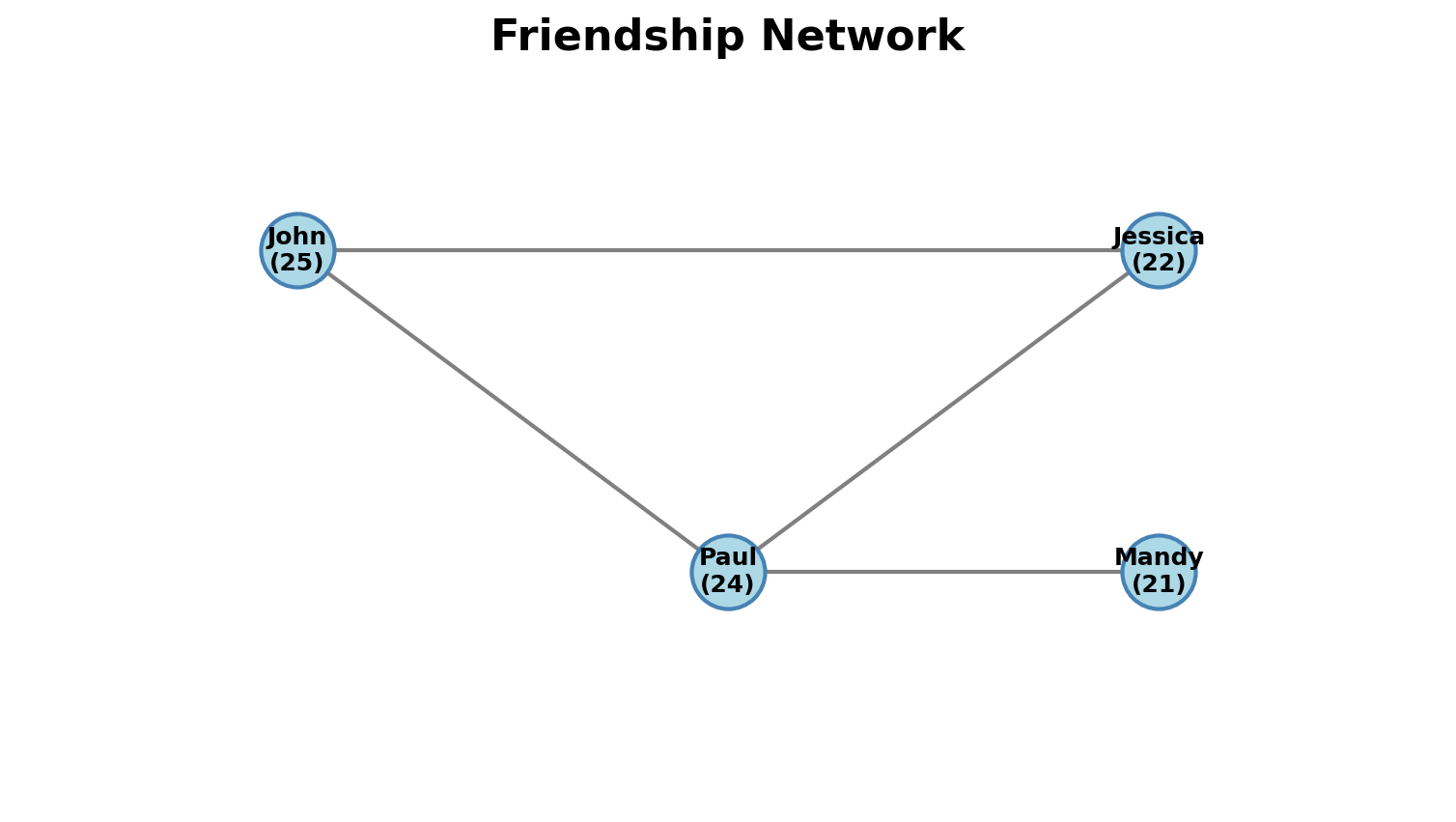{width=60%} - **Nodes**: People with attributes (name, age) - **Edges**: Friendship connections - **Attributes**: Could encode strength, duration, message count ::: notes - Concrete example to ground abstract concepts - This is undirected (friendship is mutual) - Later: directed graphs (Twitter follows, citations) - Question: "How would you find the most connected person?" ::: --- ## Fundamental Approaches ::: {.columns} ::: {.column width="60%"} **1. Node-Link Diagrams** - Nodes = dots/markers - Edges = connecting lines - Two types: Force-directed (algorithmic) & Fixed (meaningful positions) **2. Adjacency Matrices** - Rows & columns = nodes - Cells = edges - No line crossings, but less intuitive ::: ::: {.column width="40%"} 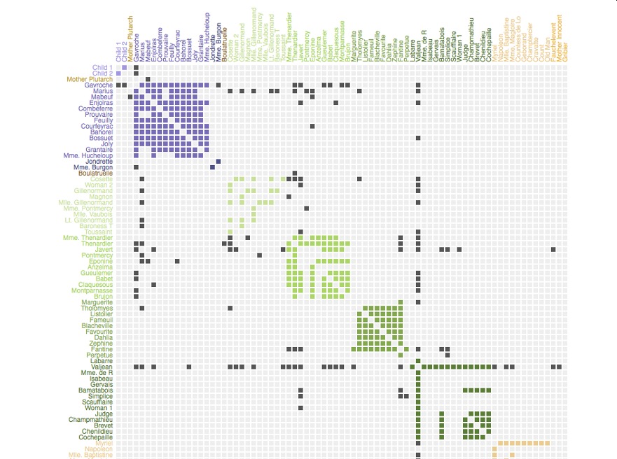 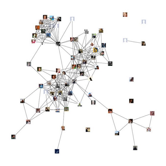 ::: ::: ::: notes - Two fundamental paradigms - trade-offs between them - Node-link: Intuitive, shows structure, but clutters - Matrix: Scalable, precise, but unfamiliar ::: --- # Force-Directed Layouts Physics simulation for automatic positioning --- ## Force-Directed: How It Works ::: {.columns} ::: {.column width="50%"} **Physical Analogy**: - **Edge Attraction**: Connected nodes pull together (springs) - **Node Repulsion**: All nodes push apart (charged particles) - System evolves until forces balance **Result**: Clusters emerge, bridges visible, hubs toward center ::: ::: {.column width="50%"} 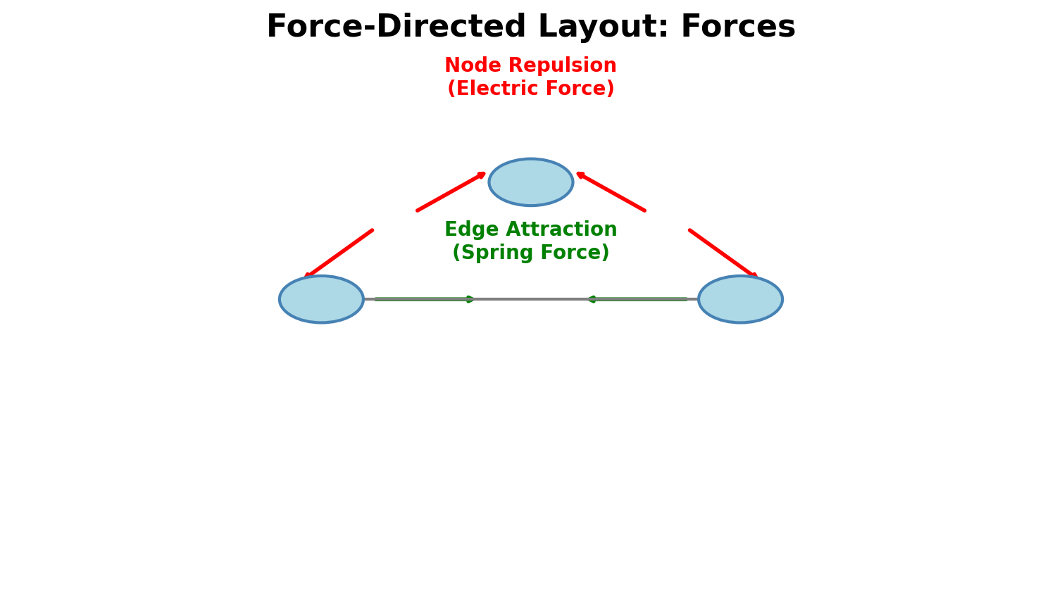 ::: ::: ::: notes - Treat network as physical system - let physics arrange it - NOT "correct" layout (networks have no inherent positions) - BUT: Often reveals meaningful structure - Many variants: Fruchterman-Reingold, Kamada-Kawai, ForceAtlas2, D3 force ::: --- ## Force-Directed Algorithm ::: {.columns} ::: {.column width="50%"} **Steps**: 1. **Initialize**: Random positions 2. **Calculate**: Net force on each node (attraction + repulsion) 3. **Move**: Displace nodes by force × step_size 4. **Iterate**: Repeat until convergence (50-500 iterations) **Complexity**: O(n²) per iteration (expensive for large networks) ::: ::: {.column width="50%"} 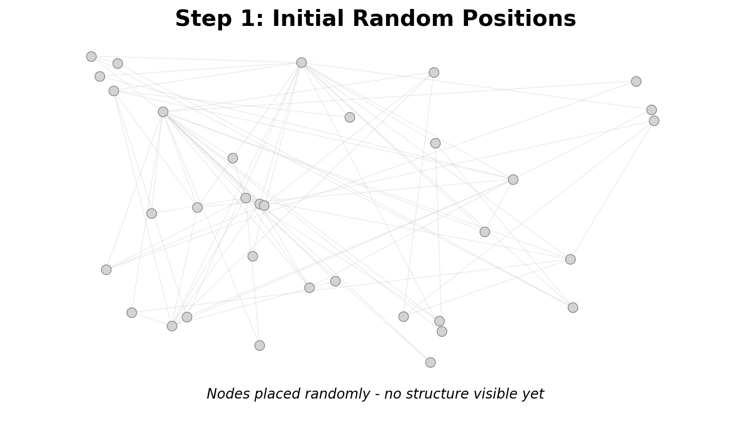{height=200px} 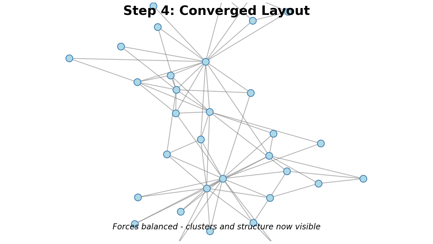{height=200px} ::: ::: ::: notes - Start: Chaos (random dots) - End: Structure (organized, balanced) - Convergence criteria: low energy, max iterations, or negligible changes - Modern optimizations use Barnes-Hut for O(n log n) ::: --- ## Visual Encoding on Nodes & Edges ::: {.columns} ::: {.column width="50%"} **Node Encodings**: - **Size**: Degree, importance, value - **Color**: Category, cluster, metric - **Shape**: Type (circles, squares, triangles) **Edge Encodings**: - **Thickness**: Weight, strength, traffic - **Pattern**: Type (solid, dashed, dotted) - **Color**: Category, direction ::: ::: {.column width="50%"} 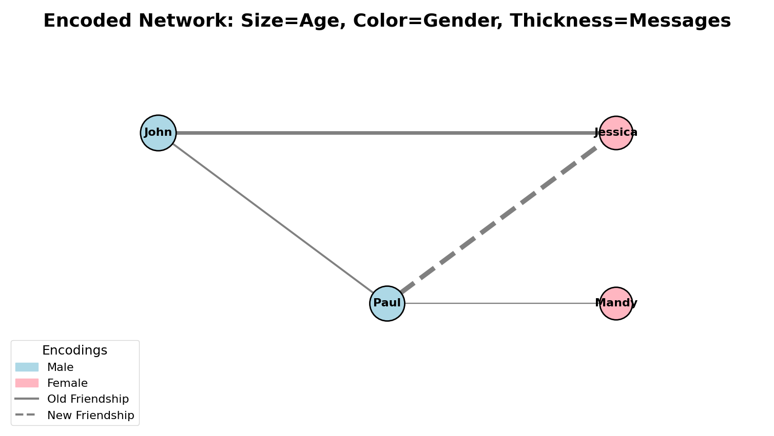 **Example**: Size=age, Color=gender, Thickness=messages, Pattern=old/new friendship ::: ::: ::: notes - Force-directed gives positions, but we have more visual channels! - Link back to perception lectures: Visual channel hierarchy - Warning: Don't over-encode (too complex = unreadable) - Example shows 4 encodings - approaching the limit ::: --- # Fixed Layouts Meaningful node positions instead of algorithmic --- ## Fixed Layouts: When & Why **When to use fixed instead of force-directed**: 1. Nodes have meaningful attributes for positioning (geography, time, hierarchy) 2. Emphasizing edges/flows more than clustering 3. Need stable, reproducible layouts **Common patterns**: Circular, linear, grid, spatial (geographic) {width=70%} ::: notes - Fixed = WE decide positions (not algorithm) - Trade structure visibility for semantic positioning - Example: Geographic networks (airports at real locations) ::: --- ## Circular Layouts & Edge Bundling ::: {.columns} ::: {.column width="50%"} **Circular Layout**: - Nodes evenly distributed around circle - **Critical decision**: Node ordering (alphabetical? by cluster? to minimize crossings?) **Edge Bundling**: - Route similar edges along common paths - Reduces clutter, reveals flow patterns ::: ::: {.column width="50%"}  ::: ::: :::footer Holten, D. (2006). [*Hierarchical edge bundles*](https://doi.org/10.1109/TVCG.2006.147). IEEE TVCG. ::: ::: notes - Node order matters! Different orders reveal different patterns - Edge bundling: Trade individual edge traceability for overall flow visibility - Holten's 2006 paper hugely influential - thousands of citations ::: --- ## Spatial Networks & Bundling ::: {.columns} ::: {.column width="50%"} **Geographic Networks**: Nodes at real locations (airports, cities, servers) **Problem**: Edge clutter! **Solution**: Edge bundling reveals corridors, hubs, regional patterns **Tools**: qGIS, Gephi, D3.js ::: ::: {.column width="50%"}   ::: ::: :::footer ::: ::: notes - Classic example: European flight network - Before: Spaghetti! Can't see anything - After: Major travel corridors, hub cities visible - Use when aggregate patterns > individual connections ::: --- # Adjacency Matrices Table representation of networks --- ## Matrices: Concept & Trade-offs ::: {.columns} ::: {.column width="50%"} **Encoding**: - Rows & columns = nodes - Cell (i,j) = edge from node i to j - Color/symbol = edge weight/presence **Advantages**: ✓ All nodes visible, ✓ No crossings, ✓ Scalable to denser networks **Disadvantages**: ✗ Less intuitive, ✗ Needs reordering, ✗ n² space, ✗ Hard to trace paths ::: ::: {.column width="50%"} 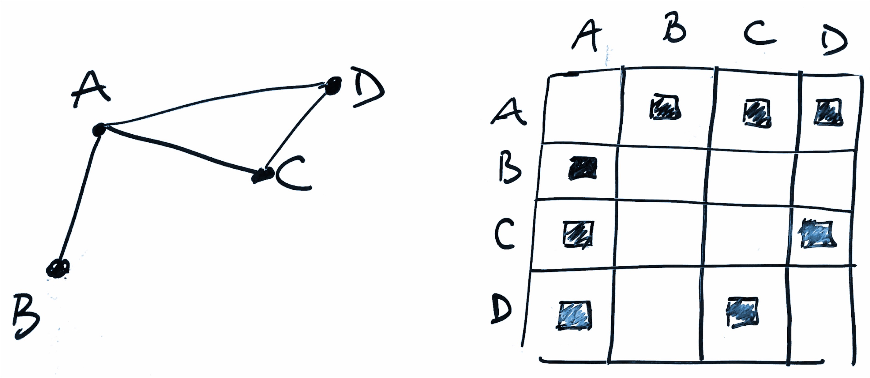 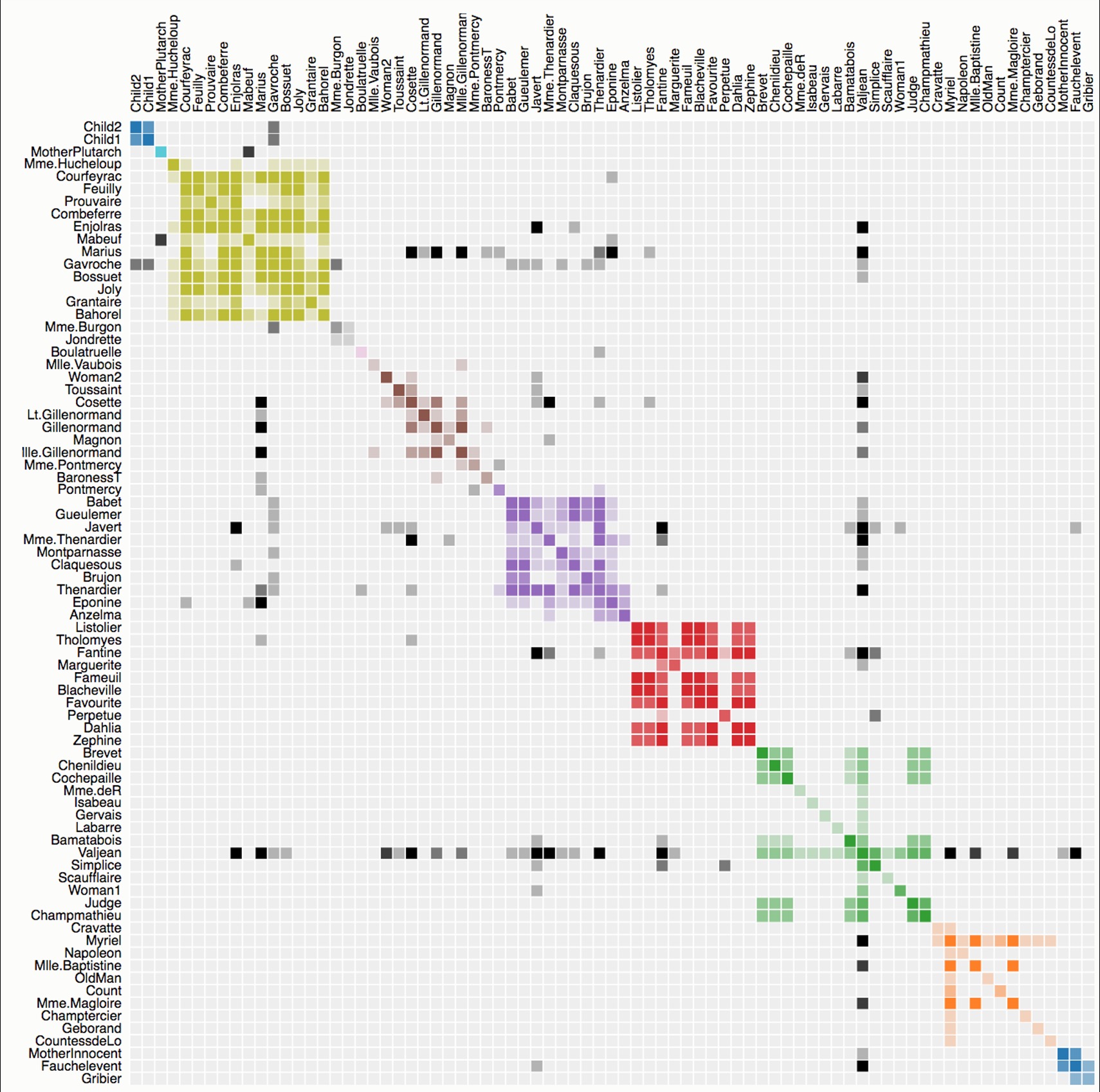{height=300px} ::: ::: ::: notes - Completely different paradigm from node-link - User studies: Experts faster with matrices, novices prefer node-link - Task matters: Degree queries easier with matrices, path queries easier with node-link ::: --- ## The Hairball Problem & Matrix Ordering ::: {.columns} ::: {.column width="50%"} **"Hairball"**: Dense networks as node-link diagrams = unreadable **Solution**: Switch to matrix OR apply clutter reduction **Critical**: Matrix ordering reveals patterns! ::: ::: {.column width="50%"} 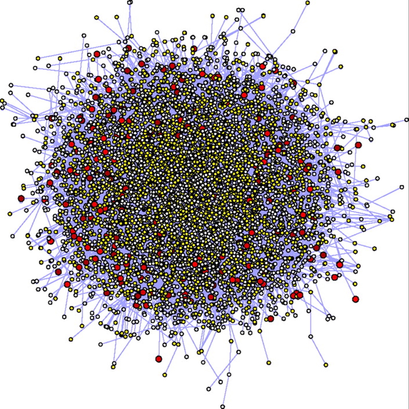{height=250px} 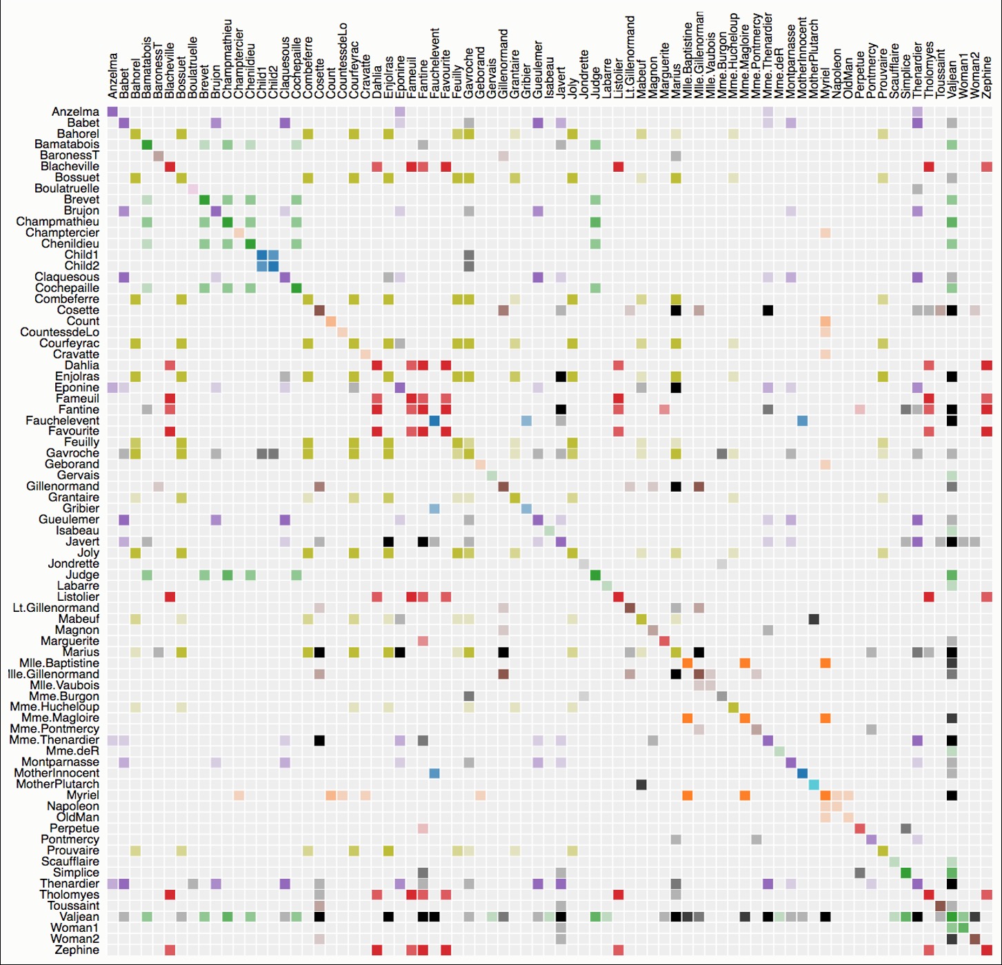{height=150px} 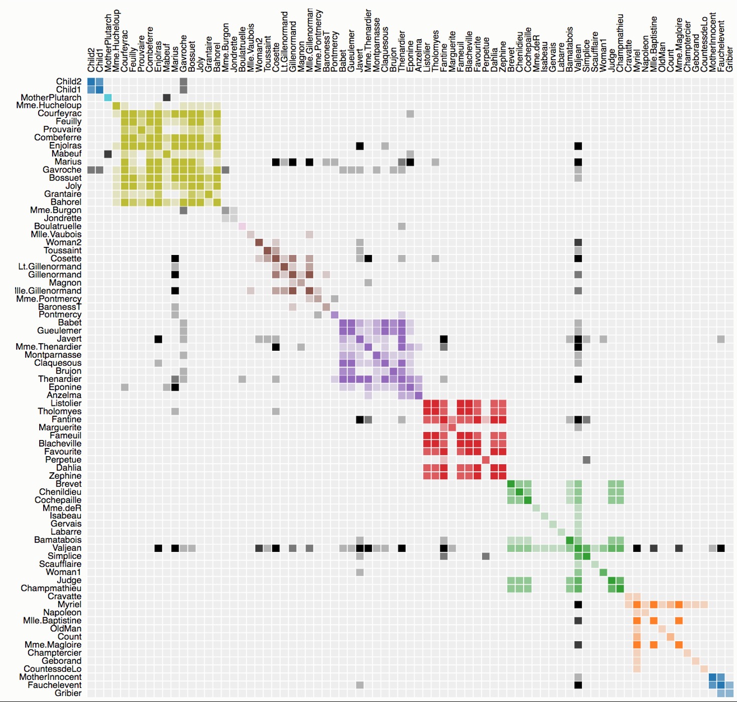{height=150px} ::: ::: ::: notes - Hairball = technical term for unreadable dense node-link - Ordering is critical design parameter (like aspect ratio for line charts) - Strategies: alphabetical, by degree, clustering, seriation algorithms - NP-hard to find optimal ordering ::: --- ## Directed Graphs & Alternatives ::: {.columns} ::: {.column width="50%"} **Directed Matrices**: - Asymmetric: (i,j) ≠ (j,i) - Above diagonal = one direction - Below diagonal = opposite direction - Easy to see reciprocity **Alternative**: Parallel axes (bipartite-like view) ::: ::: {.column width="50%"} 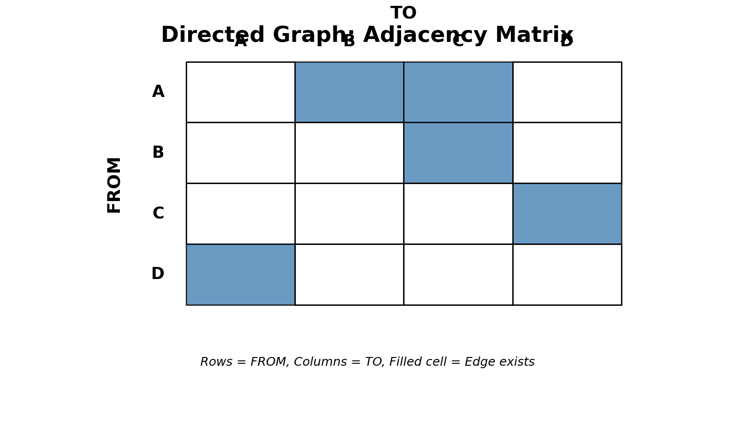 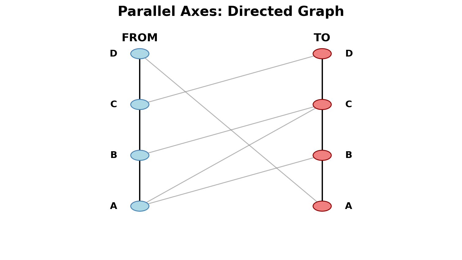 ::: ::: ::: notes - Directed graphs: Twitter follows, citations, email, transactions - Matrix naturally handles direction (no overlapping arrows) - Parallel axes: Compact, shows in/out degree, but edges cross ::: --- ## Clutter Reduction Strategies ::: {.columns} ::: {.column width="60%"} **Five main techniques**: 1. **Edge Bundling**: Route similar edges together 2. **Clustering**: Group nodes into super-nodes 3. **Filtering**: Show subset (threshold, top-k, backbone) 4. **On-Demand**: Show edges only on hover/click 5. **Motif Simplification**: Replace patterns with glyphs (cliques, stars → symbols) ::: ::: {.column width="40%"} 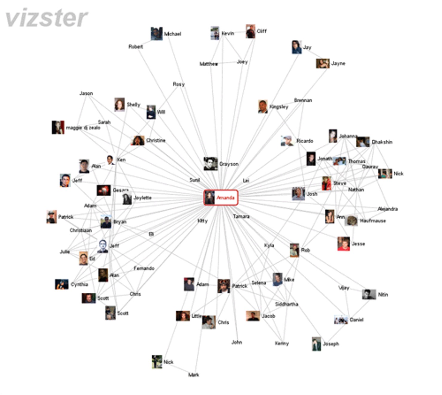{height=200px} 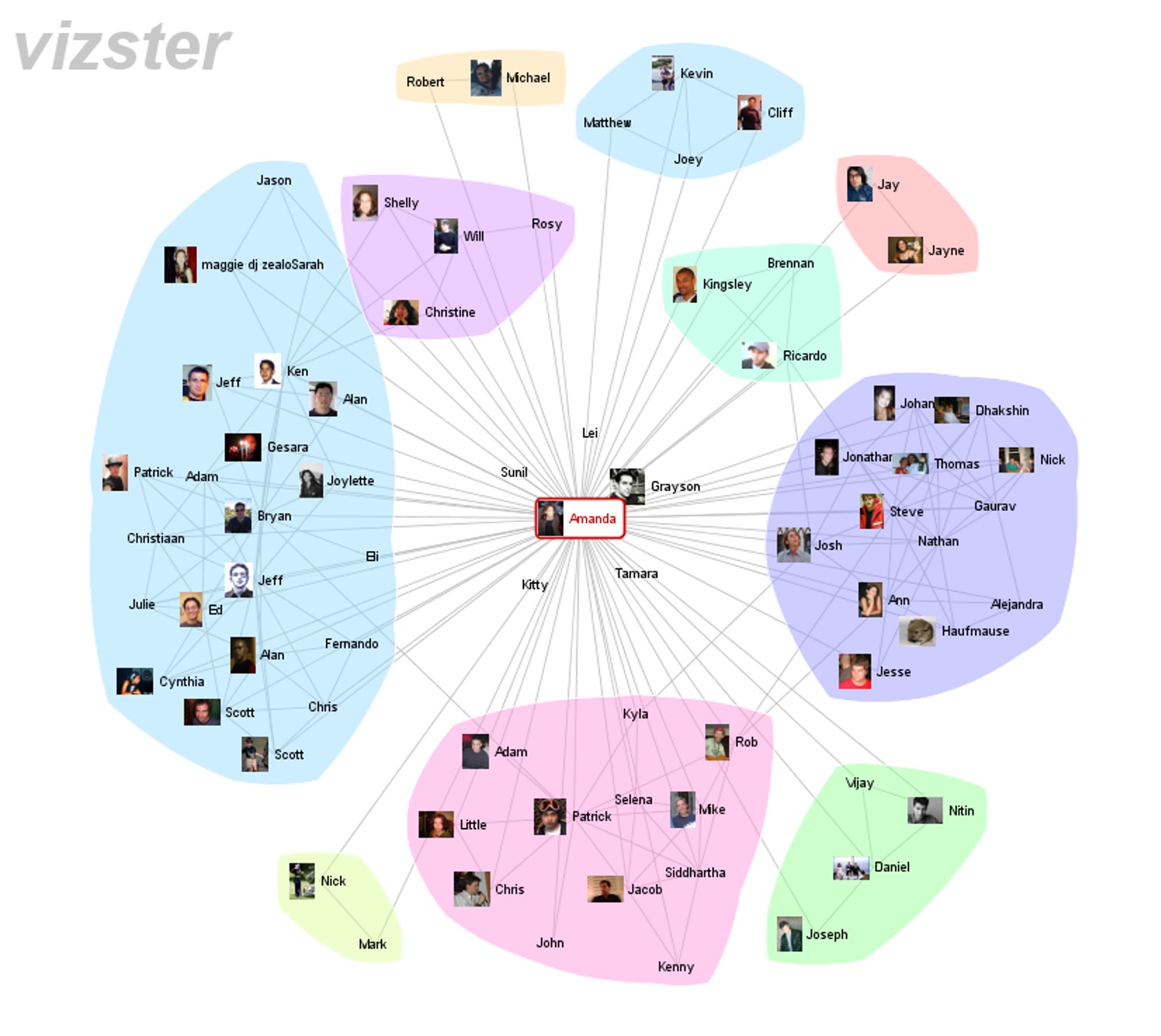{height=200px} ::: ::: :::footer Dunne, C., & Shneiderman, B. (2013). [*Motif simplification*](https://doi.org/10.1145/2470654.2466444). CHI. ::: ::: notes - Dense networks need strategies to make them comprehensible - Often combine multiple techniques (bundle + cluster + filter) - Trade detail for clarity - Best practice: Progressive disclosure (overview → drill-down) ::: --- ## Quiz: Fixed vs Force-Directed **Question**: The main advantage of a fixed layout over force-directed is: A. Less cluttered visualizations B. Node positions encode meaningful data C. Faster computation **Answer**: B - Position can carry information (geography, time, category) ::: notes - A is wrong: Fixed can be MORE cluttered (many crossings) - C is true but not the MAIN advantage (speed is secondary) - B is correct: The key benefit is semantic positioning - Choose fixed when attributes > structure ::: --- # Part 2: Trees (Hierarchies) Specialized networks with no cycles --- ## Trees: Definition & Applications ::: {.columns} ::: {.column width="50%"} **Tree**: Network with hierarchical structure, no cycles **Properties**: - One **root** node - **Parent-child** relationships - **Leaves**: Nodes with no children - Unique path between any two nodes **Real-world**: File systems, org charts, evolutionary trees, taxonomies, syntax trees ::: ::: {.column width="50%"} 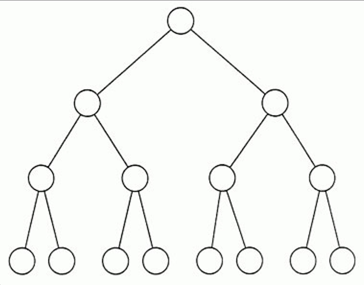 ::: ::: ::: notes - Trees are everywhere! One of most fundamental data structures - Hierarchy is natural way humans organize information - Reduces cognitive load (can't remember 10,000 items, but can remember 7±2 categories with subcategories) - This motivates specialized visualization techniques ::: --- ## Two Approaches for Trees ::: {.columns} ::: {.column width="50%"} **1. Node-Link** - Explicit parent-child connections - Structure very visible - Familiar, intuitive - **Limitation**: Doesn't scale (exponential width growth) 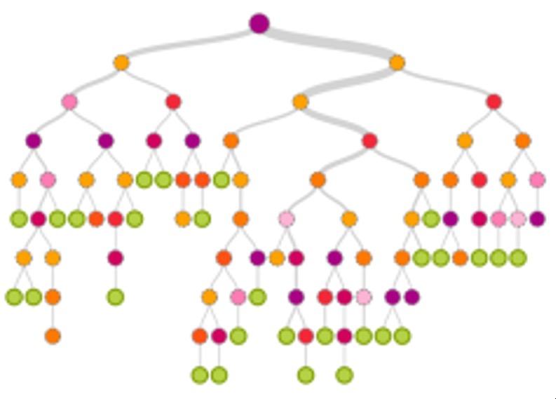 ::: ::: {.column width="50%"} **2. Space-Filling (Containment)** - Nesting shows hierarchy - No explicit edges - Space-efficient, can show size - **Limitation**: Structure harder to see 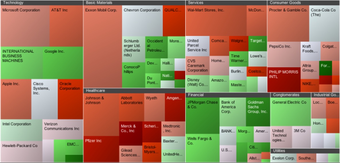 ::: ::: ::: notes - Fundamental trade-off: Structure vs Scalability - Node-link: Good for small trees (<100 nodes) - Space-filling: Good for large trees (1000s of nodes) ::: --- ## Node-Link Trees: Examples ::: {.columns} ::: {.column width="33%"} **Top-Down** 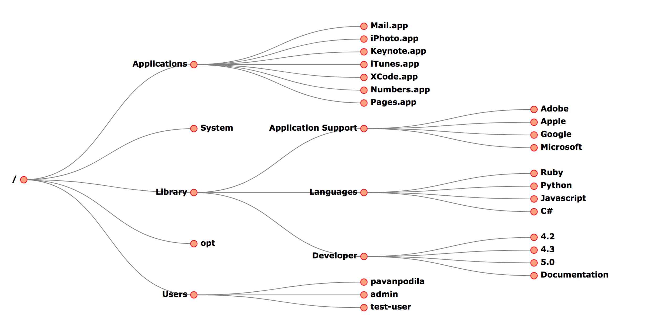 File systems, org charts ::: ::: {.column width="33%"} **Radial** 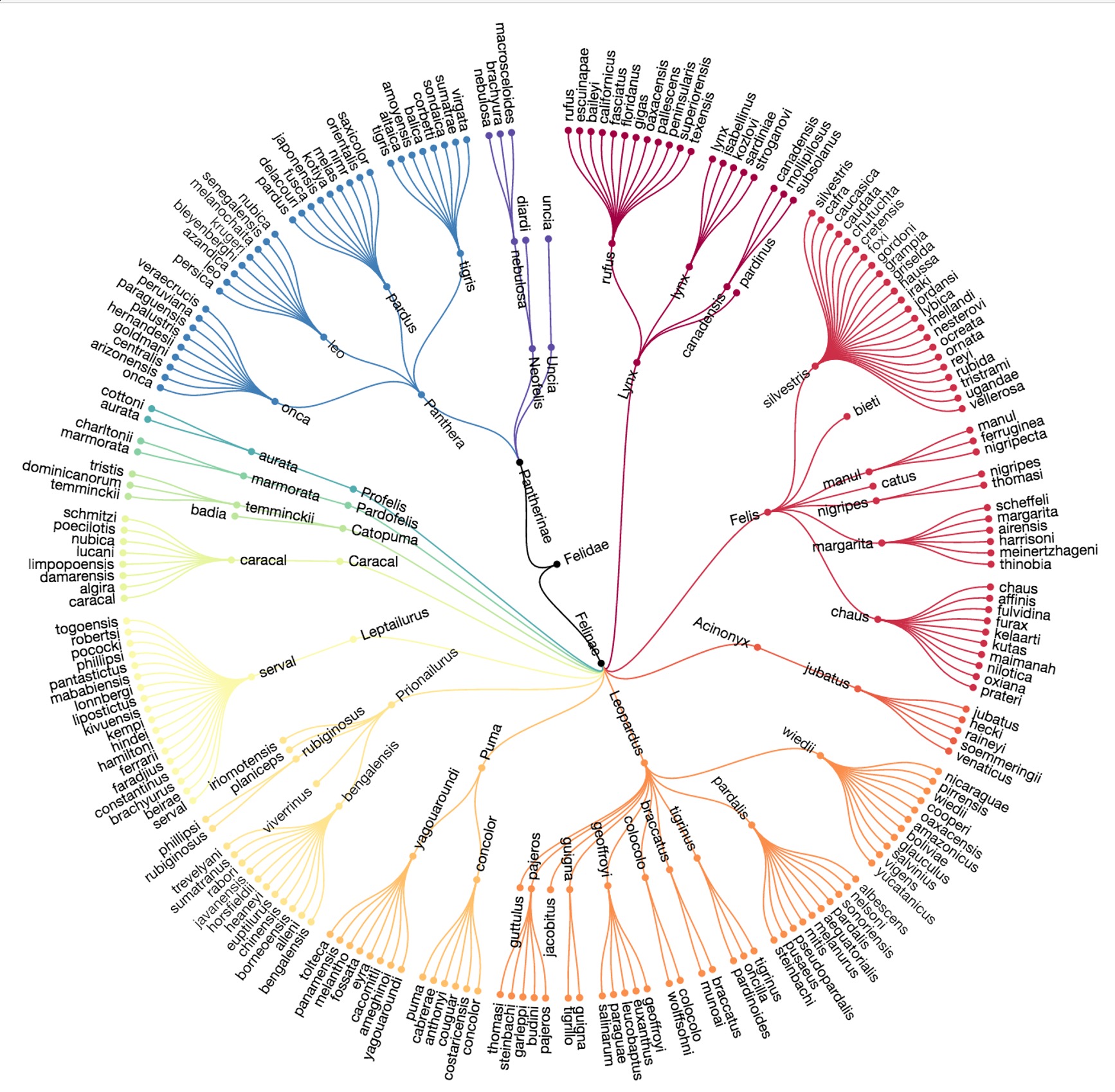 More space-efficient ::: ::: {.column width="33%"} **Indented List** 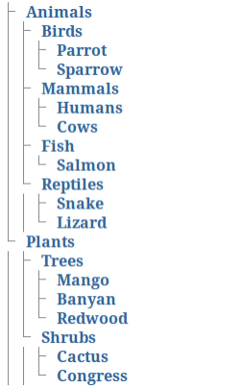 Most compact ::: ::: **Issues**: Scalability (1D growth), labeling, limited encoding channels ::: notes - Top-down: Most familiar, matches mental model - Radial: Uses 2D space radially, aesthetically pleasing - Indented: Most compact, used in file browsers - All struggle with large/deep trees ::: --- ## Special Trees: Dendrograms ::: {.columns} ::: {.column width="50%"} **Dendrogram**: Tree showing hierarchical clustering results **Algorithm** (Agglomerative): 1. Start: Each point = own cluster 2. Find two closest clusters 3. Merge them (height = distance) 4. Repeat until one cluster **Properties**: - Binary tree structure - Branch height = dissimilarity at merge - Cutting at height defines # of clusters **Used in**: Gene expression, customer segmentation, document clustering ::: ::: {.column width="50%"} 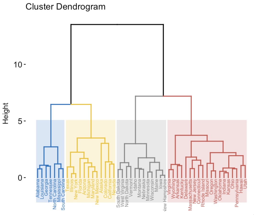 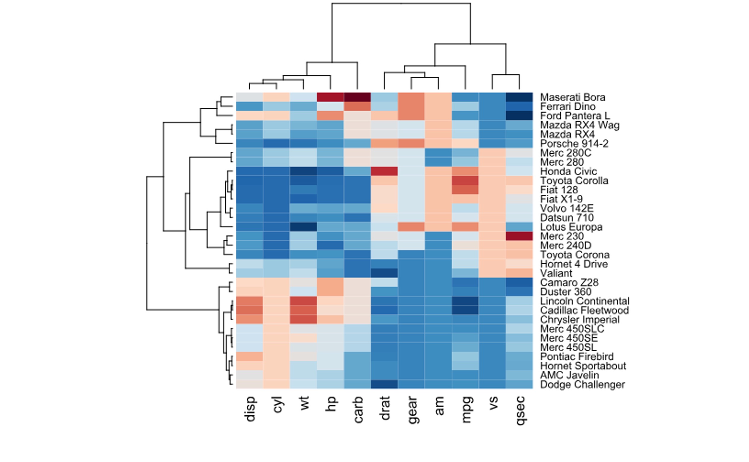 ::: ::: ::: notes - Specific type of tree from hierarchical clustering algorithm - Branch height is meaningful (unlike layout-only trees where height is just for layout) - Algorithm is bottom-up: Start with individual points, iteratively merge closest clusters - Height at which clusters merge represents their dissimilarity - Cutting dendrogram horizontally at different heights gives different numbers of clusters - Often paired with heatmaps for multivariate data (shown in image) - Standard in biology, but useful across any domain where you can define distance/similarity - Example: Gene expression (cluster genes by similar expression patterns) ::: --- ## Special Trees: Decision Trees ::: {.columns} ::: {.column width="50%"} **Decision Tree**: Each node = decision point **Two contexts**: 1. Human decision-making (flowcharts, election scenarios) 2. Machine learning (learned classification models) **Why visualize**: Interpretability, debugging, trust, bias detection ::: ::: {.column width="50%"} 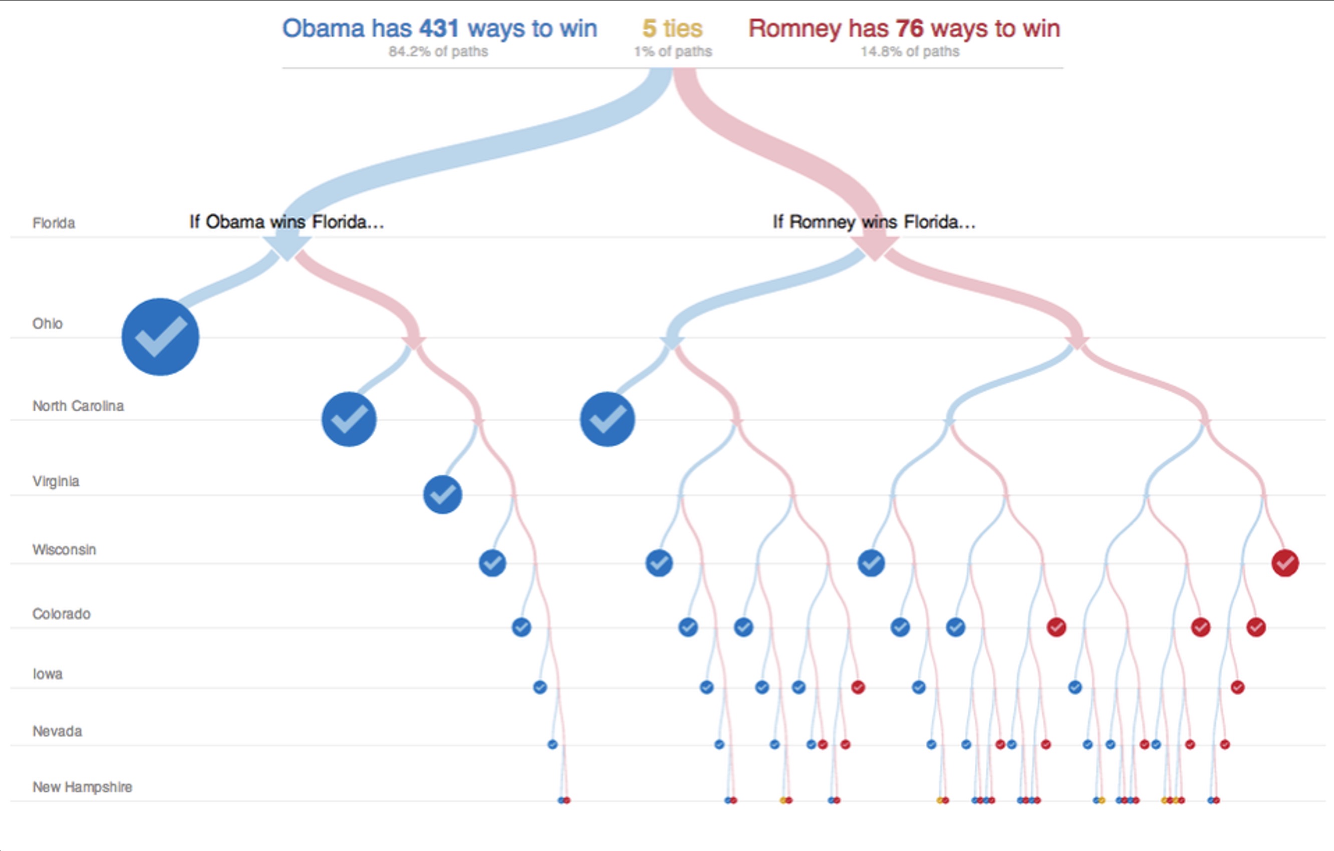 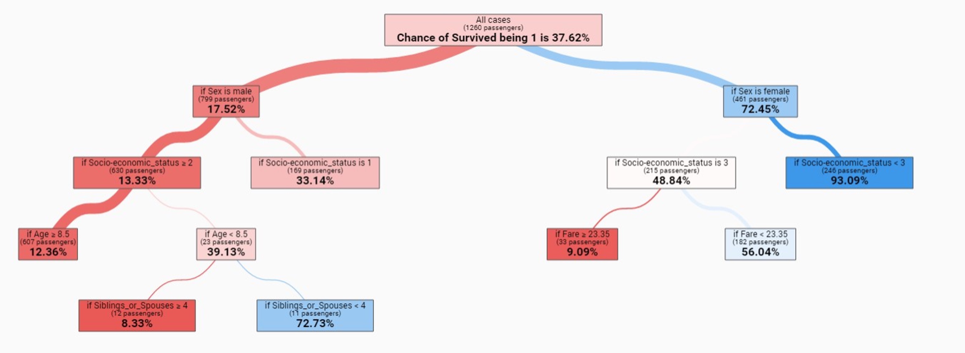 ::: ::: ::: notes - NYT 512 Paths: 2012 election scenarios (9 swing states, 2⁹=512 outcomes) - ML trees: Algorithm learns rules from data (split on attributes) - Unlike neural nets, you can SEE the model! (Explainable AI) - Used in medicine, finance, criminal justice (require transparency) ::: --- # Treemaps Space-filling approach for large hierarchies --- ## Treemaps: Origin & Encoding ::: {.columns} ::: {.column width="50%"} **Origin** (Ben Shneiderman, 1990): "My hard disk is full - what's using space?" **Encoding**: - **Area**: Quantitative value (size, revenue, count) - **Color**: Category OR secondary metric - **Nesting**: Hierarchical structure **Key innovation**: Shows BOTH hierarchy AND size ::: ::: {.column width="50%"} {height=250px} 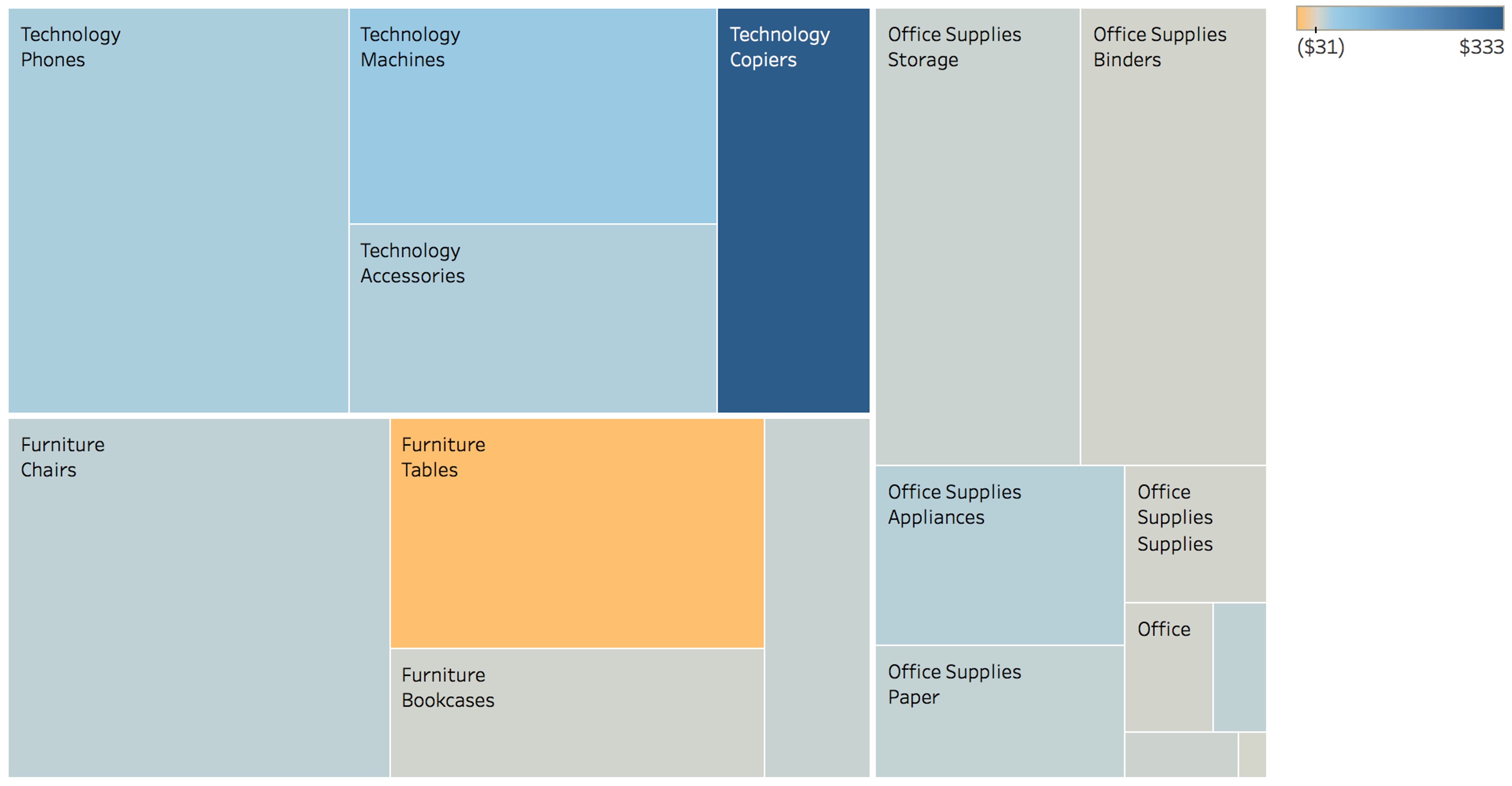 ::: ::: :::footer Shneiderman, B. (1992). [*Tree visualization with tree-maps*](https://doi.org/10.1145/102377.115768). ACM TOG. ::: ::: notes - Solving personal frustration → major innovation (5000+ citations) - Area proportional to value, sum of children = parent - Widely adopted: WinDirStat, DaisyDisk, Google Analytics, finance - Can show 1000s of nodes (limited by screen resolution, not algorithm) ::: --- ## Treemap Algorithms: Squarified vs Slice-and-Dice ::: {.columns} ::: {.column width="50%"} **Problem**: Slice-and-Dice creates thin rectangles (bad aspect ratios) **Solution**: Squarified algorithm optimizes for square-like shapes **Trade-off**: Squarified is more readable but less stable (layout changes with data updates) ::: ::: {.column width="50%"} 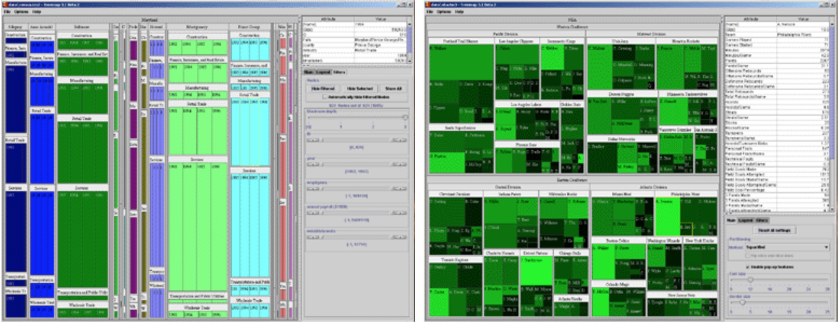 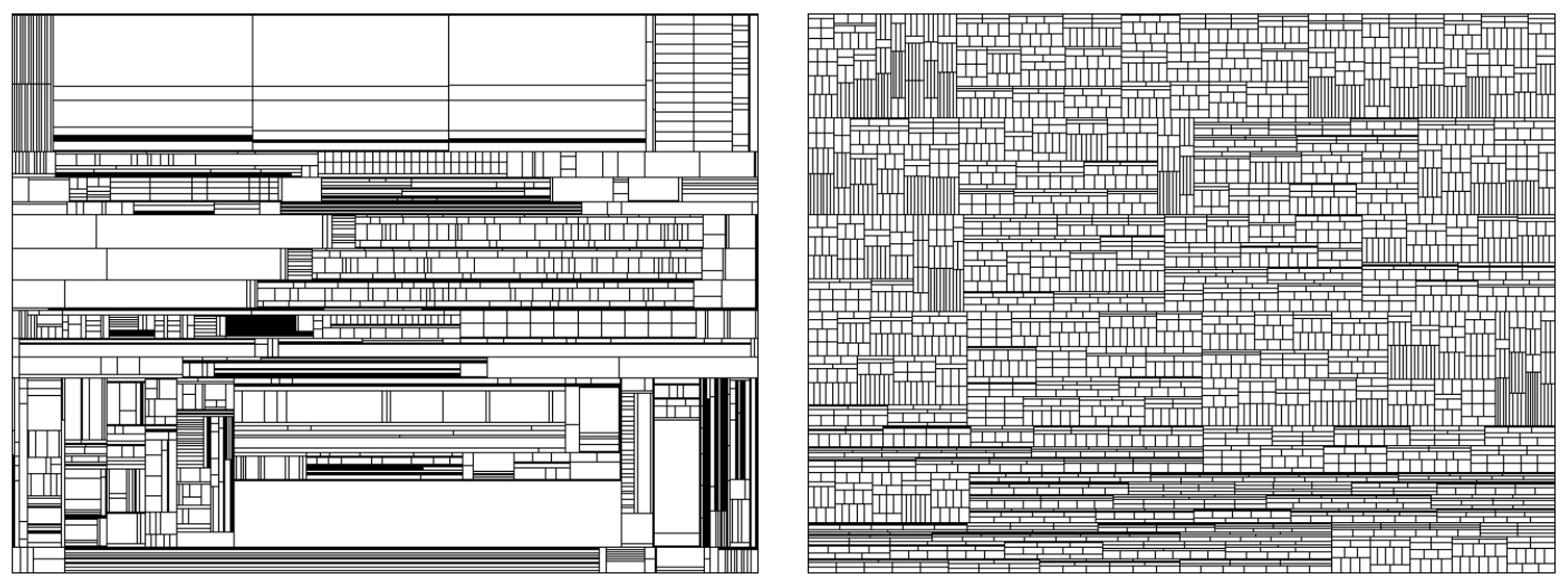 ::: ::: :::footer Bruls, M. et al. (2000). [*Squarified treemaps*](https://doi.org/10.1007/978-3-7091-6783-0_4). Springer. ::: ::: notes - Perceptual research: Squares easier to compare than elongated rectangles - Squarified: Greedy algorithm, local optimization of aspect ratios - Use squarified for single snapshots, ordered treemaps for comparisons over time ::: --- ## Treemap Examples ::: {.columns} ::: {.column width="33%"} **File Systems**  Disk usage tools ::: ::: {.column width="33%"} **Finance** 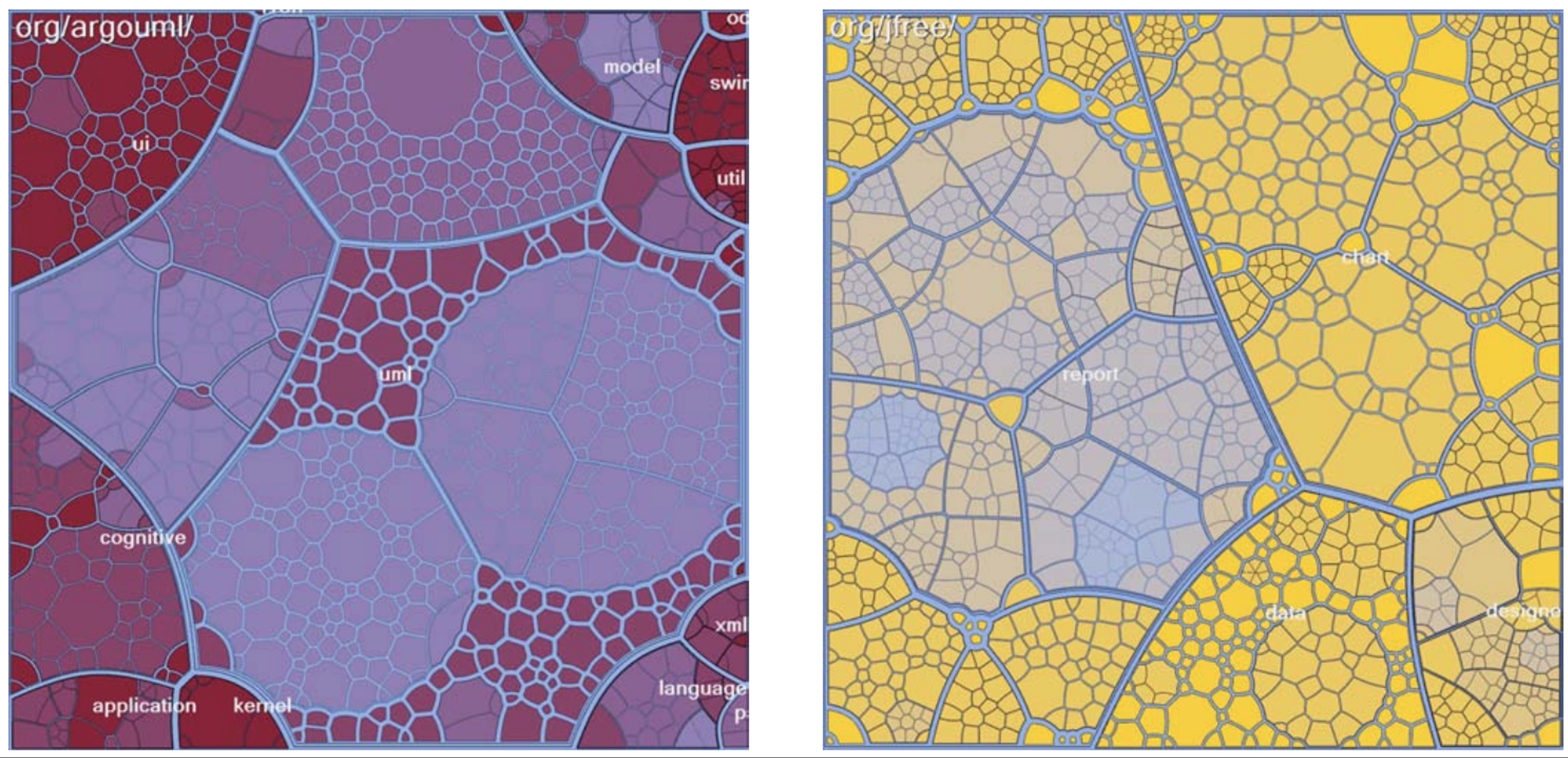 Stock market heat maps ::: ::: {.column width="33%"} **Code Analysis** 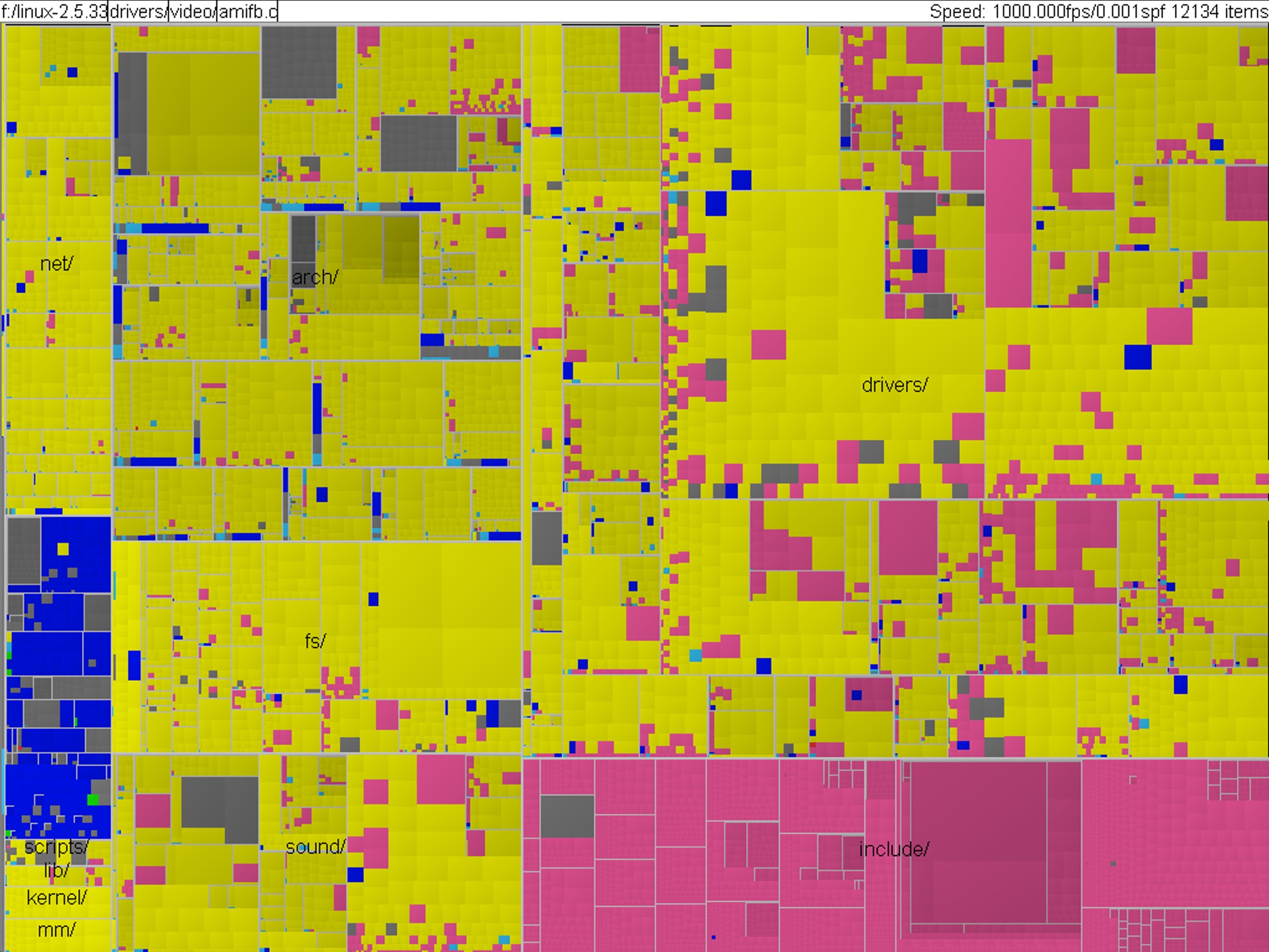 Linux kernel by file type ::: ::: **Applications**: Business dashboards, news (Newsmap), analytics, sports ::: notes - Stock markets: Area=market cap, color=% change, grouped by sector - Code: Area=file size, color=file type, reveals codebase structure - Interaction: Zoom, hover for details, search/filter ::: --- ## Treemap Trade-offs ::: {.columns} ::: {.column width="50%"} **Advantages**: - ✓ Scalability (thousands of nodes) - ✓ All nodes visible - ✓ Encodes size + category - ✓ Space-efficient **Disadvantages**: - ✗ Size less accurate than position - ✗ Structure harder to see - ✗ Layout algorithm affects readability ::: ::: {.column width="50%"} 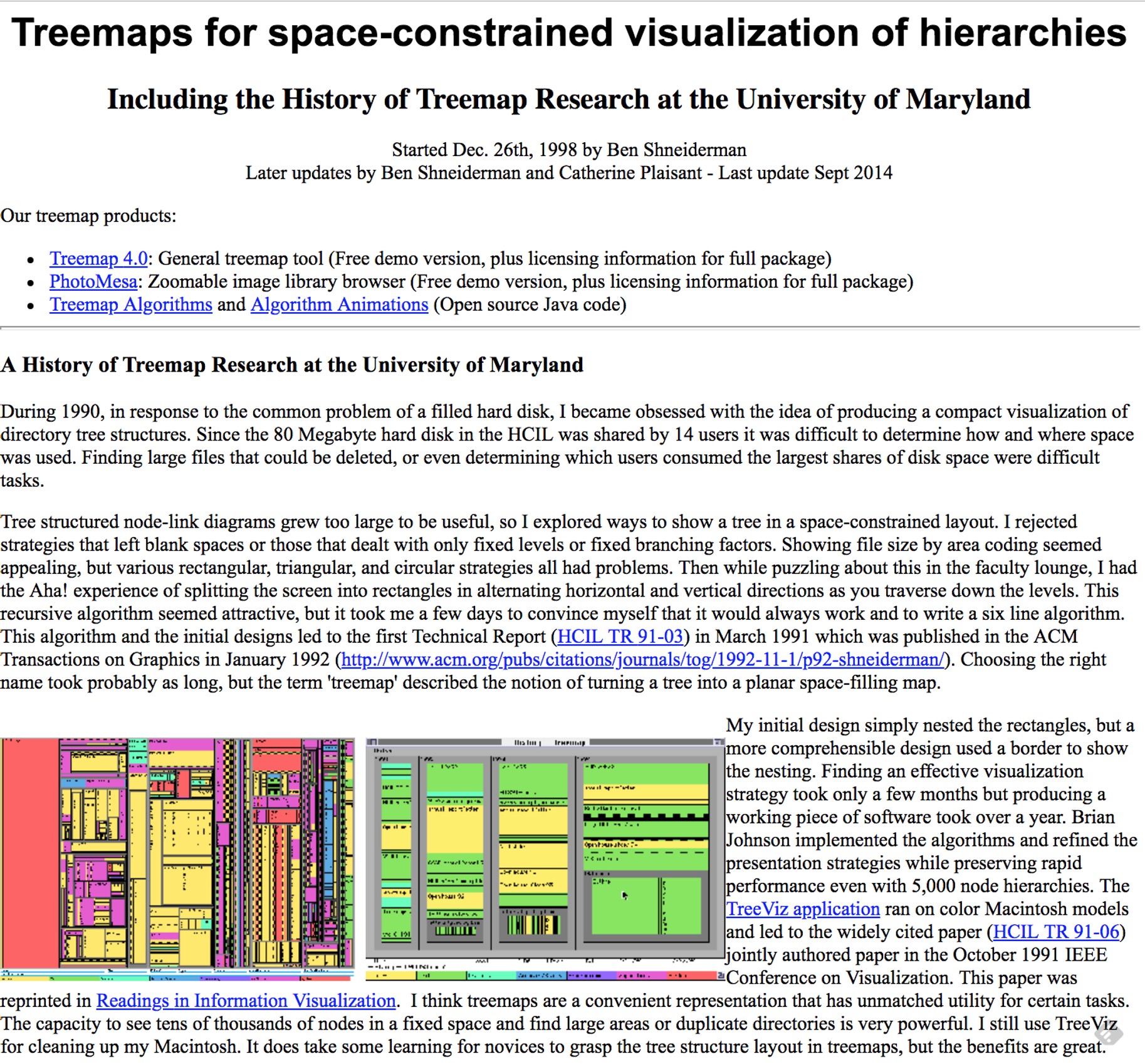 ::: ::: ::: notes - **When to use**: - Large hierarchies (>100 nodes) - Quantitative data at leaves (size matters) - Need magnitude comparisons - **When NOT**: - Small trees (<50 nodes) → node-link clearer - Structure more important than size - No meaningful quantitative attribute ::: --- ## Sunburst & Icicle Plots ::: {.columns} ::: {.column width="50%"} **Middle ground** between node-link and treemaps: - **Sunburst**: Radial (concentric rings) - **Icicle**: Linear (horizontal bands) **Space efficiency**: Treemap > Icicle > Sunburst **Hierarchy perception**: Icicle ≈ Sunburst > Treemap **Familiarity**: Treemap > Icicle > Sunburst ::: ::: {.column width="50%"} 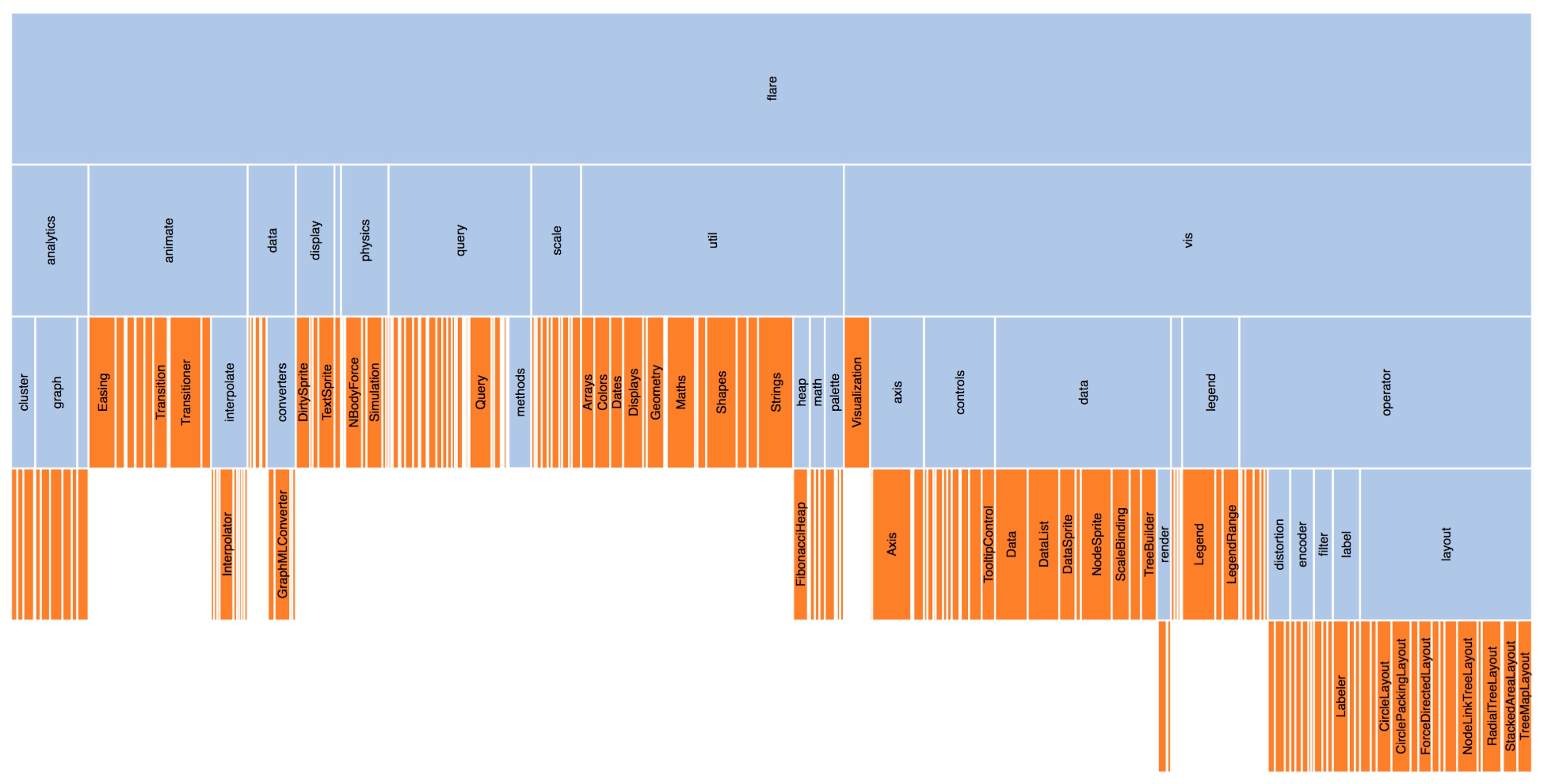 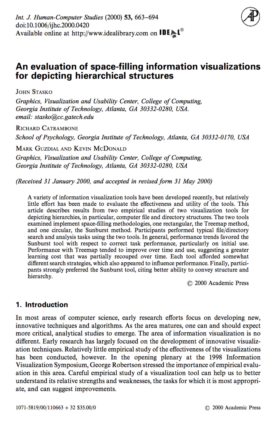 ::: ::: ::: notes - Use when both structure AND size matter - Sunburst: Beautiful, angle=proportion, radius=depth - Fixed height/width per level (less efficient than treemaps) - Growing in popularity with interactive zoomable versions ::: --- # Summary & Recommendations --- ## Visualization Method Summary **Networks (General Graphs)**: - **Force-Directed**: Unknown structure, exploration, <100 nodes - **Fixed Layout**: Known groupings, spatial data, semantic positioning - **Matrix**: Dense networks, analytical tasks, expert users **Trees (Hierarchies)**: - **Node-Link**: Small trees (<100), structure focus, intuitive - **Treemaps**: Large trees (1000s), size focus, space-efficient - **Sunburst/Icicle**: Balance of structure + size, moderate depth **Key principle**: No single "best" method - depends on data, task, audience ::: notes - Data size drives choice (sparse vs dense, small vs large) - Task matters (structure vs values, paths vs clusters, overview vs details) - Audience matters (experts vs general public, static vs interactive) - Often use multiple views with linking ::: --- ## Design Guidelines & Trade-offs **Key dimensions to consider**: 1. **Clutter**: How crowded? 2. **Scalability**: How many nodes/edges? 3. **Structure visibility**: How clear is topology? 4. **Familiarity**: How intuitive for audience? 5. **Reordering needs**: Preprocessing required? **Decision process**: Try multiple approaches → prototype → user test → iterate ::: notes - No perfect visualization - all involve trade-offs - Clutter: Node-link high (dense graphs), Matrix low - Scalability: Node-link ~100, Matrix ~1000, Treemap ~10,000 - Structure: Force-directed high, Fixed low (unless meaningful) - Best practice: Prototype multiple, use linked views, provide interaction ::: --- ## Programming Exercises (suggestion!) **Create variants of each technique**: 1. **Force-directed layout**: Implement algorithm OR use D3.js, experiment with encodings 2. **Circular/chord diagram**: Fixed layout with edge bundling 3. **Node-link tree**: Top-down OR radial, with collapse/expand 4. **Treemap**: Squarified algorithm with zoom/drill-down **Explore**: - Visual encodings (size, color, thickness) - Interaction (zoom, filter, details-on-demand) - Real datasets (social, citations, file systems, hierarchical clustering) **Tools**: D3.js, Gephi, Cytoscape, NetworkX (Python), igraph (R) ::: notes - Encourage: Implement from scratch (learn algorithms) AND use libraries (practical) - Datasets available: Course website, Gephi sample data, D3 examples - Focus on design decisions (encodings, interaction, layout parameters) ::: --- ## Resources & References **Essential readings**: - Shirley Wu: [*Understanding the Force*](https://medium.com/@sxywu/understanding-the-force-ef1237017d5) - Holten (2006): *Hierarchical Edge Bundling* - IEEE TVCG - Shneiderman (1992): *Tree Visualization with Tree-maps* - ACM TOG - Bruls et al. (2000): *Squarified Treemaps* - Springer **Advanced topics**: Motif simplification (Dunne & Shneiderman), semantic substrates, time-varying networks, multilayer networks **Interactive examples**: Observable (D3.js), Gephi tutorials, Graph visualization survey papers ::: notes - Shirley Wu's article is THE best force-directed tutorial - Holten & Shneiderman papers are foundational (must-reads) - Observable has live, editable examples (great for learning) - Encourage exploration of tools (Gephi for analysis, D3 for custom viz) ::: --- ## Thank You! **Next class**: Week 14 - Final Project Presentations **Questions?** ::: notes - Key takeaways: - Two paradigms: Node-link vs Matrix - Trees enable specialized techniques - Always consider: Data, Task, Audience - Prototype multiple approaches - Interaction overcomes static limitations - Office hours: Available for project help - Reminder: Programming assignments + readings :::