Urban Visualization I

Flows, Time & Interactivity (2D + Time) - CS-GY 6313 - Fall 2026

Claudio Silva

2026-10-30

From Static Maps to Dynamic Urban Systems

The Yellow Blob Problem

What happens when we apply static techniques to massive urban datasets?

This is one week of NYC taxi trips (about 3.5 million) drawn as points on a map.

What can you learn from this?

Nothing. It’s a “yellow blob.”
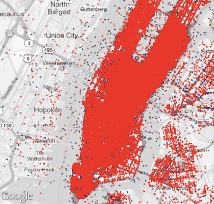
One week of NYC taxi trips drawn as points: pickups blue, dropoffs red

Today’s Goal

Learn to visualize urban dynamics—movement and time—using interactive, linked views

  • Challenge: Urban data is massive, dense, and dynamic
  • Solution: Turn visualization into an exploration tool
  • Case Study: TaxiVis—a system for exploring NYC taxi flows

We’ll learn how to move from this “yellow blob” to meaningful insights about urban mobility patterns.

Part 1: The Urban Context

Why This Matters

The Urban Challenge:

  • Over 50% of world’s population in cities
  • +2.5 billion more by 2050
  • Cities = centers of innovation
  • But also: sprawl, pollution, inequality

How do we make better decisions about urban development?

The Data Opportunity:

  • We can now collect, store, and open massive urban datasets
  • Benefits:
    • Government: Operations & planning
    • Science: Discovery
    • Residents: Participation
    • Industry: Innovation

What Makes Urban Data Unique?

Three Interacting Components:

  1. Residents - People and their behavior
  2. Infrastructure - Physical systems and policies
  3. Environment - Natural and built surroundings

To understand a city, we must explore how these interact over space and time.

Four Key Characteristics:

  1. Scale
    • Human-level to metro-level
    • Millions of individual events
  2. Density
    • Massive overplotting
    • Traditional techniques fail
  3. Complexity
    • Interconnected systems
    • Transit, traffic, social networks
  4. Dynamism
    • Cities defined by time & movement
    • Static snapshots miss the essence

Hägerstrand’s Space-Time Cube (1970)

The Classic Framework for Movement Analysis

  • X, Y dimensions: Geographic space
  • Z dimension: Time
  • Each person’s life: a line through the cube

The Urban Challenge:

Understanding millions of these paths, all interacting simultaneously
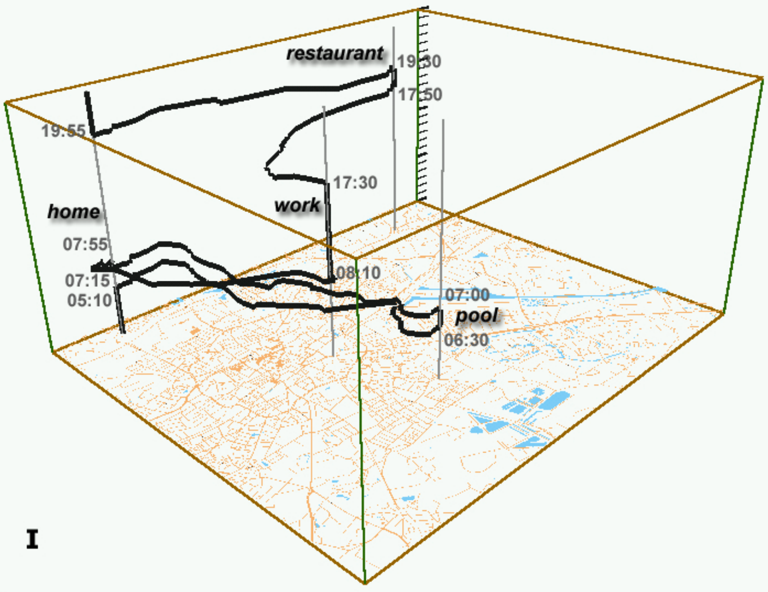
A space-time cube: one person’s day as a path through space (floor plan) and time (vertical axis)

Part 2: Why Traditional Analysis Fails

The Old Workflow (Confirmatory Data Analysis)
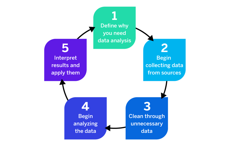
A generic five-step data analysis cycle

The Loop:

  1. Define why you need the analysis
  2. Collect data from sources
  3. Clean away unnecessary data
  4. Analyze the data
  5. Interpret the results and apply them

Every new question is another trip around the loop.

The Problems with Traditional Workflows

❌ Cognitive overload - Generates overwhelming numbers of plots/tables

❌ Batch-oriented - No exploration, just predetermined queries

❌ Distances experts from data - Requires intermediary (data scientist)

❌ Cannot scale - Modern data volumes overwhelm traditional tools

❌ Result: The “yellow blob” problem

Even simple questions require generating dozens of individual plots, each manually programmed

The Problem with Current Tools

Current practice for domain experts:

  • Load small slices into R, MATLAB, Stata, ArcGIS, Excel
  • Write SQL queries or code to analyze subsets
  • Generate individual plots manually
  • Repeat for each new question

This is tedious, slow, and limiting

Why this fails:

❌ Tools can’t handle 170M trips

❌ Requires programming/database expertise

❌ Time-consuming and frustrating

❌ Distances experts from the data

❌ Hard to explore, compare, or follow up on patterns

Part 3: The Need for Interactivity

The Paradigm Shift

Static Visualization

Role: Presentation

  • Answers questions the designer anticipated
  • Fixed perspective
  • One-way communication

Limitation: Cannot handle hundreds of millions of data points

Interactive Visualization

Role: Exploration

  • Enables users to ask their own questions
  • Dynamic perspectives
  • “Dialogue with data”

Power: Query and filter to reveal patterns

The Visual Information Seeking Mantra

“Overview first, Zoom and Filter, then Details-on-Demand”

— Ben Shneiderman (1996)

1. Overview
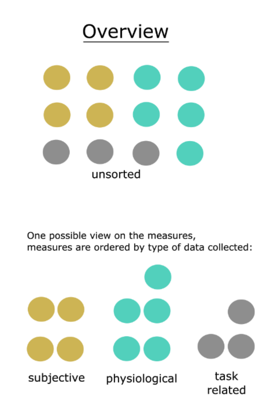
Overview: all measures, unsorted and then grouped by type

Start with the big picture (even if it’s a “yellow blob”)

2. Zoom & Filter
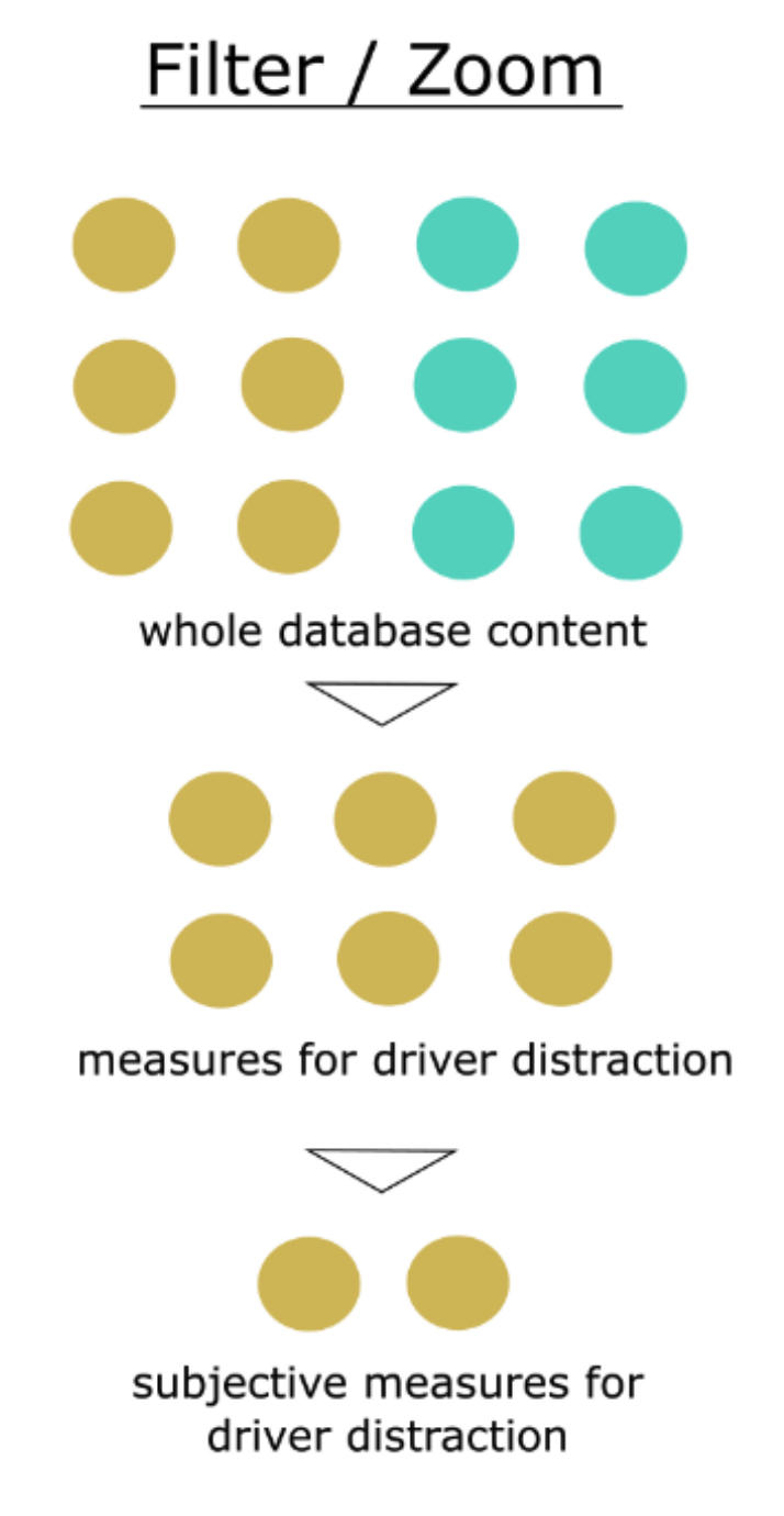
Filter: whole database narrowed to the measures of interest

Focus on items of interest

3. Details-on-Demand
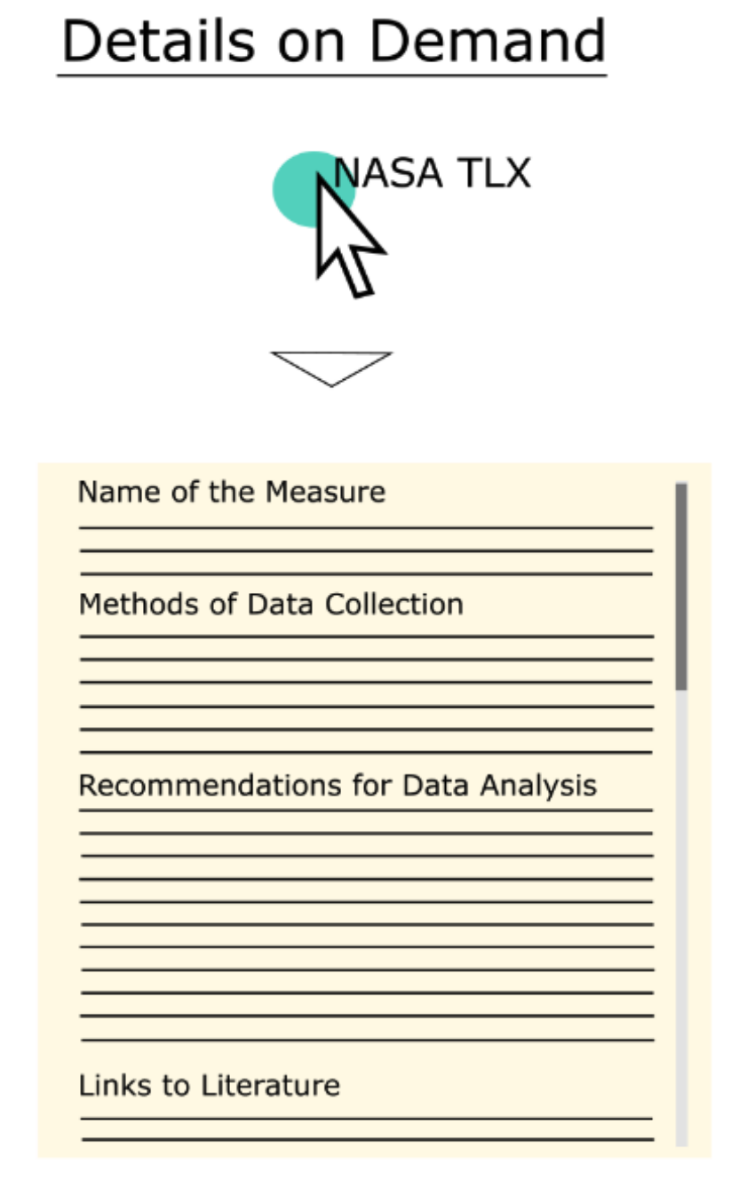
Details on demand: selecting one measure opens its record

Get specifics when needed

Why Interactivity Matters

  1. Performance is critical
    • Even 500ms latency significantly reduces exploration, observations, and hypothesis generation
    • Sub-second response enables iterative analysis
  2. Perception over cognition
    • Well-designed systems let you see patterns rather than calculate them
    • Visual queries are faster than SQL
  3. Empowers domain experts
    • No programming required
    • Direct manipulation of visualizations
    • Experts can explore data themselves

Research shows that even a half-second delay dramatically impacts analysis quality.

Part 4: Enter TaxiVis

The NYC Taxi Dataset

The Data:

  • 13,000 taxis
  • 500,000 trips/day
  • 170 million trips/year

Each trip includes:

  • Pickup/dropoff locations & times
  • Distance traveled
  • Fare amount
  • Tip amount

What can taxi data tell us?

  • Economic activity and human behavior
  • Mobility patterns across the city
  • Response to major events (hurricanes, holidays)
  • Social inequalities in service

Challenge: How do we make sense of this data?

Taxi Patterns and Anomalies

One dataset shows weekly rhythm, holiday dips, storms and street events.
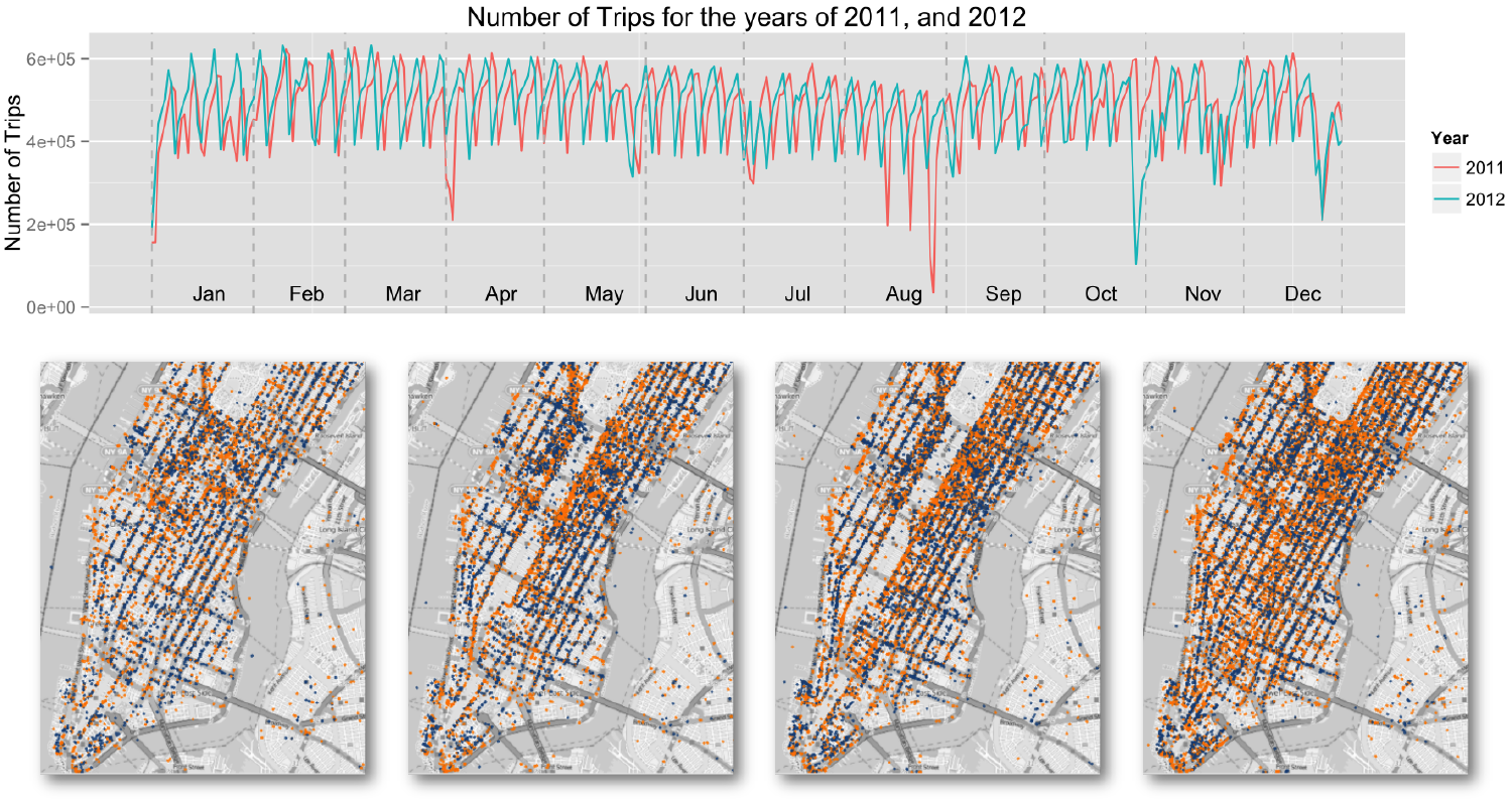
Daily taxi trips in 2011 and 2012 (top) and map snapshots of pickups and dropoffs (bottom)

Part 5: Design Requirements

What We Need (From Domain Experts)

Query Needs:

  1. Understand dynamics
    • “How do patterns vary over space and time?”
  2. Explore events
    • “What happened during Hurricane Sandy?”
  3. Compare regions
    • “Midtown vs. Harlem taxi frequency?”
  4. Study movement
    • “Where do people go from JFK?”

System Requirements:

  • Interactive - Sub-second response times
  • Expressive - Support complex spatio-temporal queries
  • Usable - No SQL or programming required
  • Scalable - Handle all 170M trips, not samples
  • Comparative - Easy to compare regions and time periods

Part 6: The Visual Query Model

Core Idea: Direct Manipulation

Let users query data through direct manipulation of visualizations

Spatial

Where?

  • Pickup regions
  • Dropoff regions
  • Draw polygons on map

Temporal

When?

  • Time ranges
  • Recurrence patterns
  • Day of week

Attribute

What?

  • Fare amount
  • Distance
  • Trip duration

Instead of writing SELECT * FROM trips WHERE..., you draw on a map

Visual Representation of Queries

A query is a set of colored constraints

  • Polygon on the map = a spatial constraint (start or end region)
  • Arrow between regions = a directional constraint (origin → destination)
  • Time widget = a temporal constraint
  • Attribute ranges = fare, distance, duration

Color ties it together

  • Each query has its own color
  • That color tags the query’s line in every chart
  • A query can be a union of simpler ones, for example a polygon plus an arrow
  • To compare, put several queries in the same view

Part 7: TaxiVis Interface

The Complete System

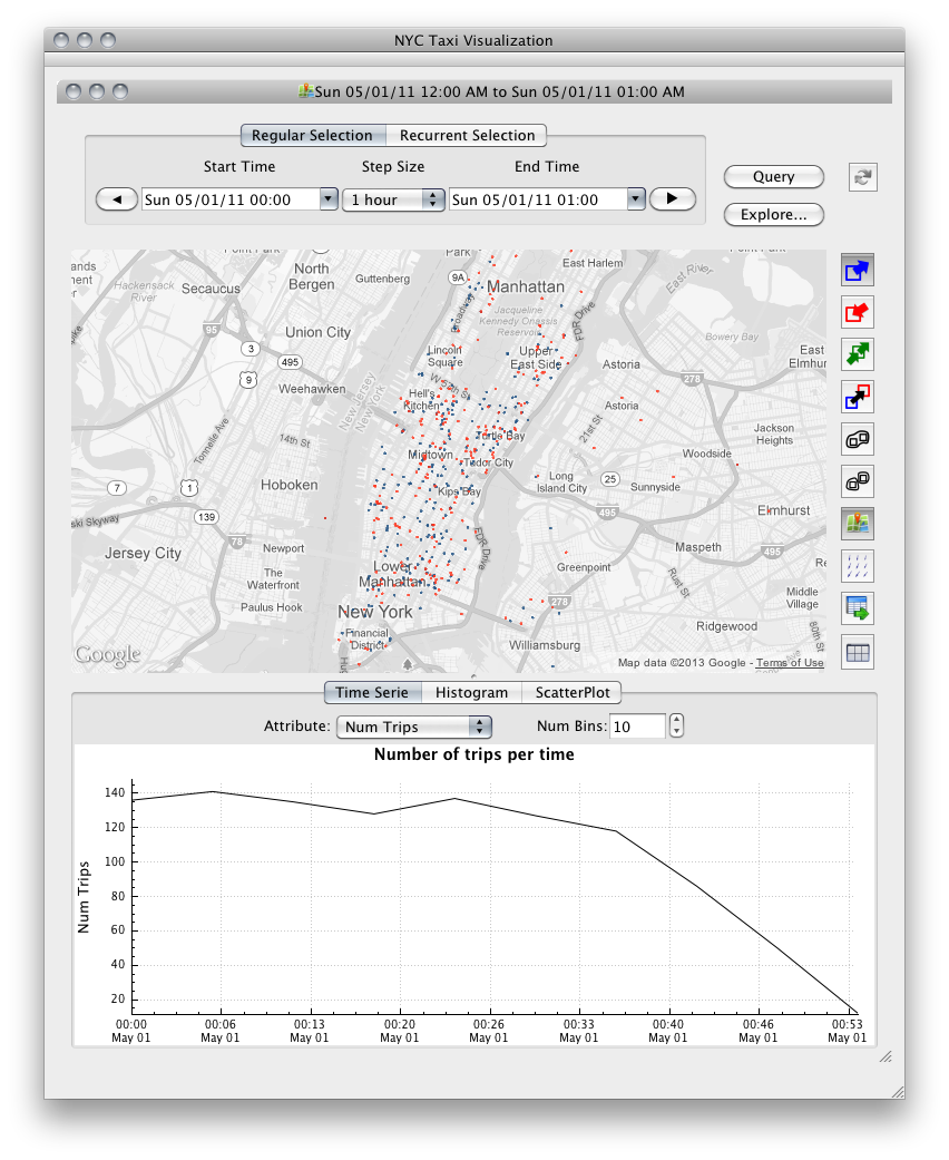
  • A. Time widget: start, end, step size; regular or recurrent selection
  • B. Map: draw polygons and arrows
  • C. Tool bar: pickups / dropoffs / both, arrows, group, export, attribute exploration
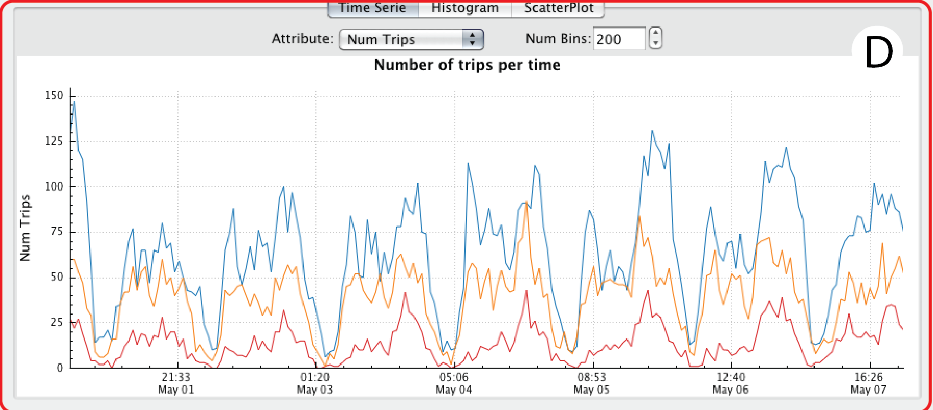
  • D. Data summary: time series, histogram or scatter plot, one line per query
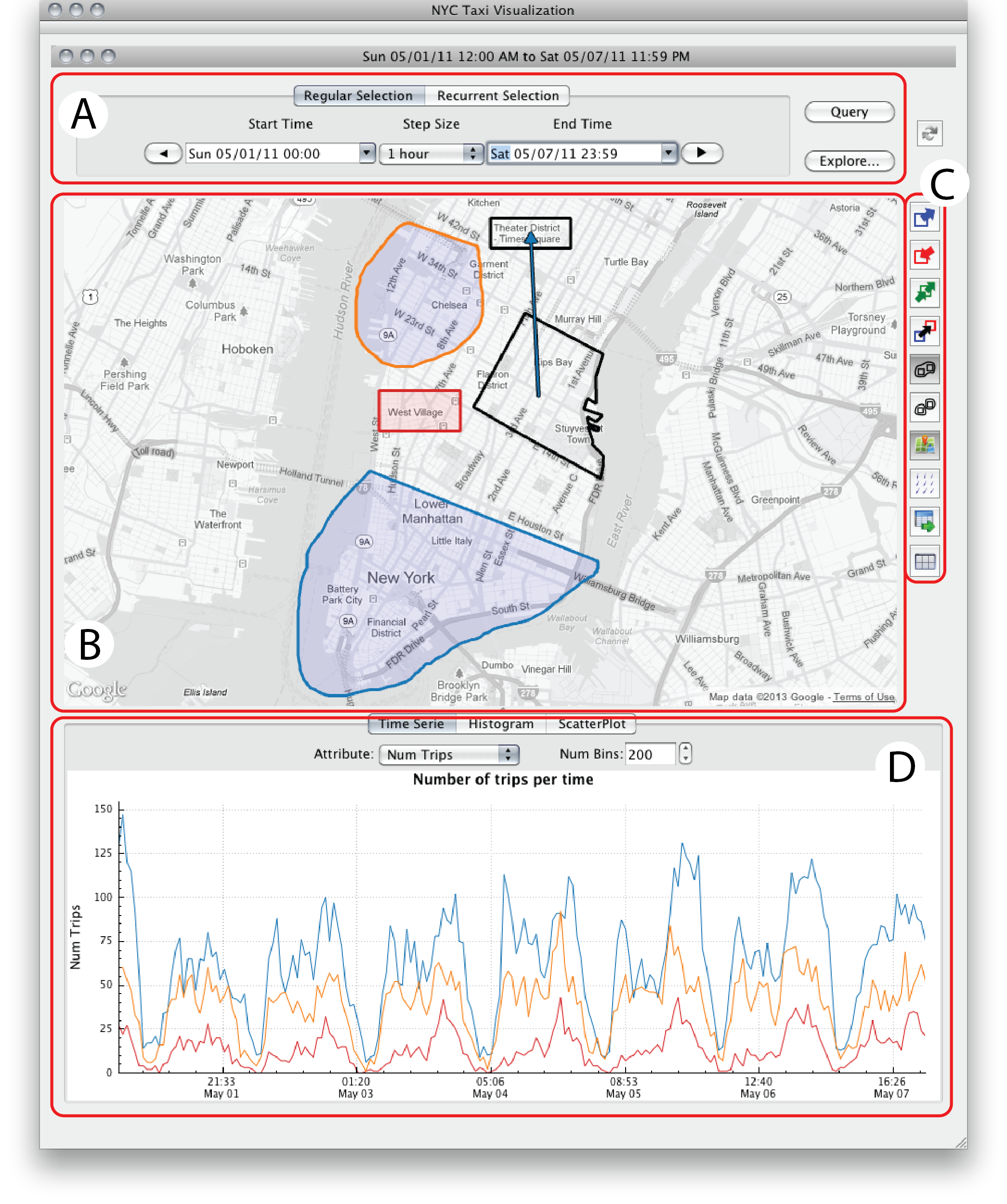
TaxiVis user interface: (A) time selection widget, (B) map, (C) tool bar, (D) data summary

Part 8: Visual Queries in Action

Example: Airport Comparison

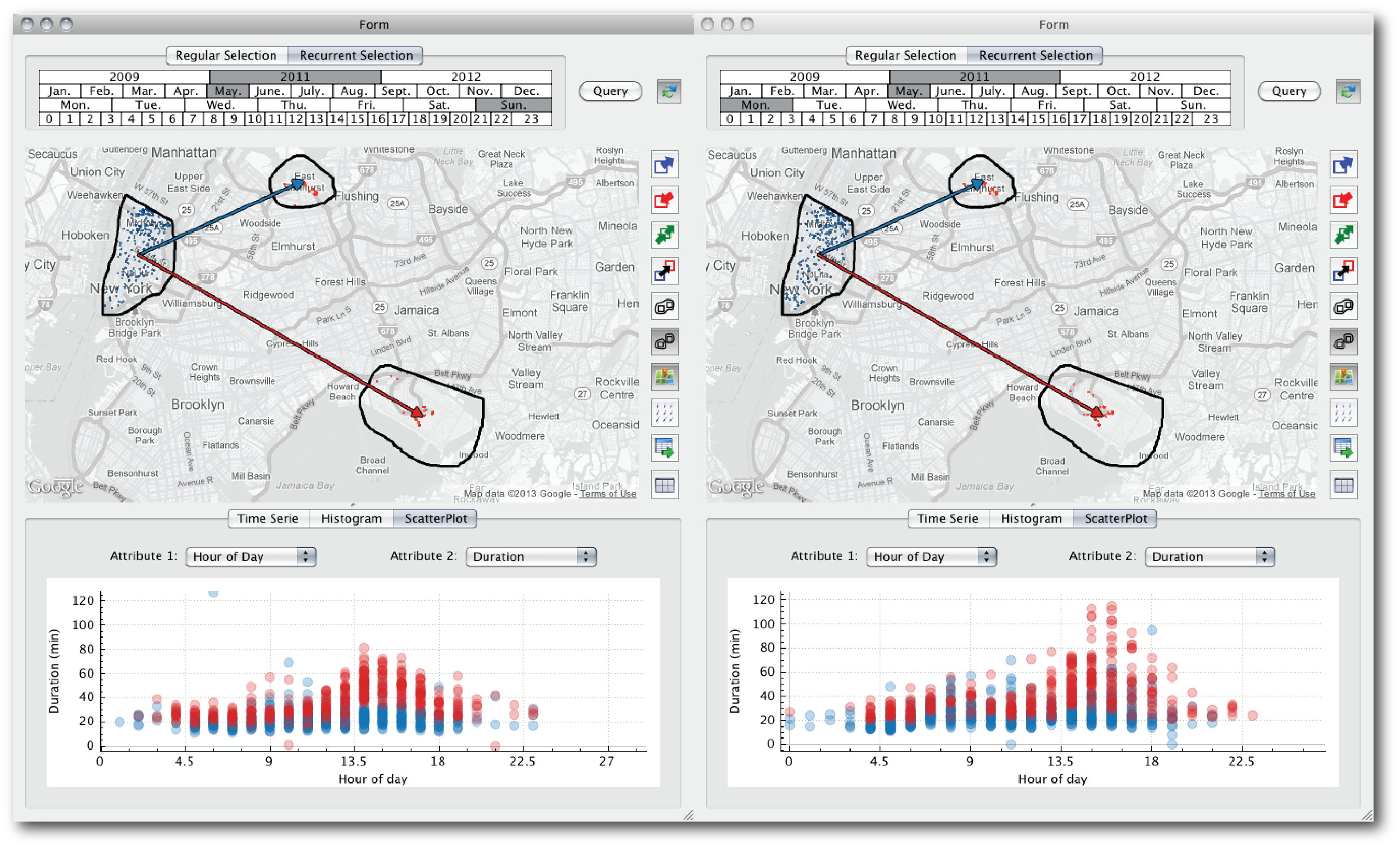
“How do trips from Manhattan to JFK and LaGuardia differ on a Sunday vs. a Monday?”
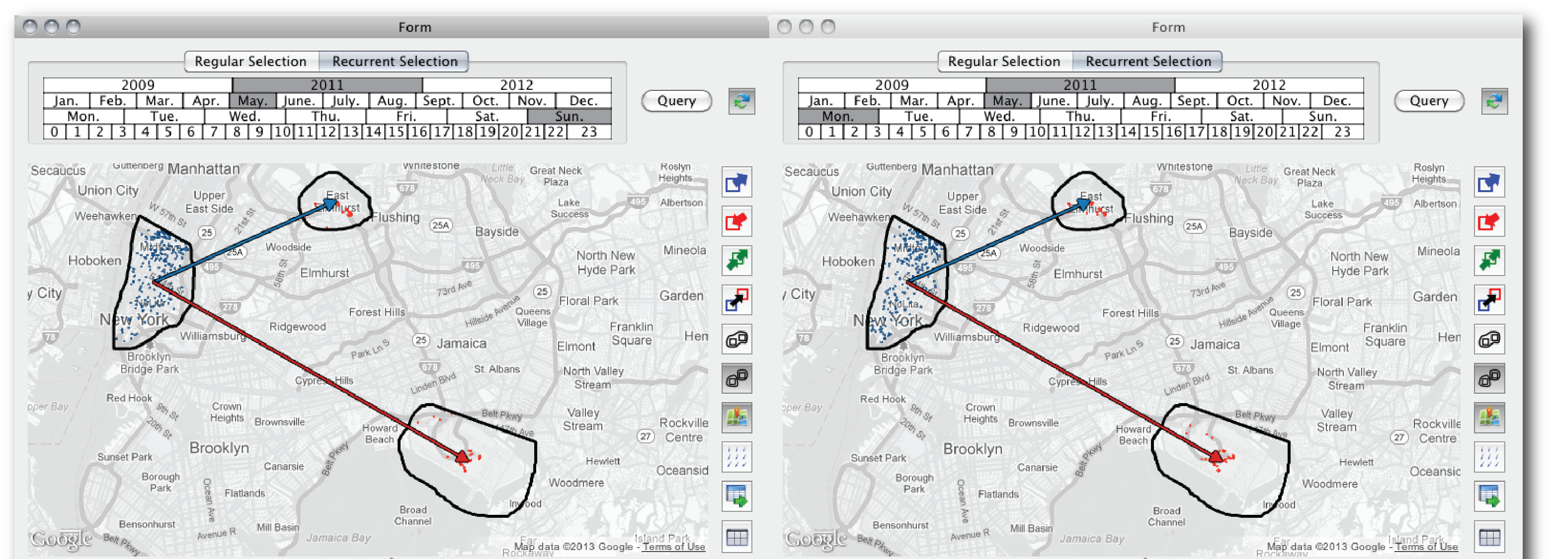
Two linked TaxiVis windows: the same Manhattan-to-airport query for Sundays (left) and Mondays (right)

The Results & Discovery
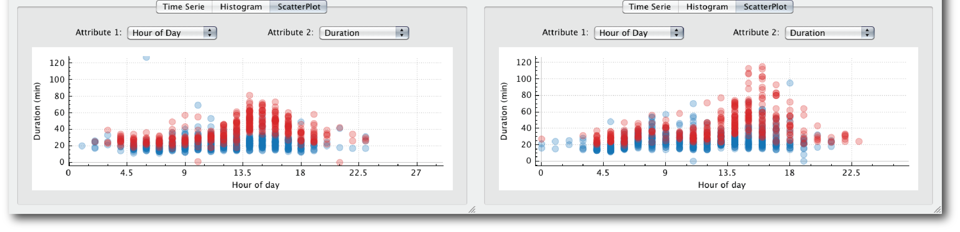
Scatter plots of trip duration against hour of day for Sundays (left) and Mondays (right); red = trips to JFK, blue = to LaGuardia
  • Each dot is a trip: hour of day vs. duration, colored like the arrows (red = JFK, blue = LGA)
  • Discovery: Monday afternoon trips to JFK are much longer, with the longest reaching about 110 minutes vs. about 80 on Sunday
  • Implication: an economic disincentive for drivers to accept airport trips

Part 9: Query Expressiveness

Peuquet’s Triad Framework

All three fundamental spatio-temporal query types:

when + where → what

“What taxis were in Midtown at rush hour?”

when + what → where

“Where were high-fare trips on New Year’s Eve?”

where + what → when

“When do trips to airports peak?”

Plus: Query Composition

  • Queries can be refined, combined, compared
  • Results can be visualized multiple ways
  • Supports both atomic queries and complex queries (unions)

Part 10: Making It Interactive

The Performance Challenge

The Problem:

  • 170M trips = traditional databases too slow
  • PostgreSQL: 24 seconds for 100k-trip query
  • SQLite: 85 seconds for same query
  • Goal: Sub-second response

The TaxiVis Solution:

  • Custom k-d tree index
    • 30GB vs. 200GB for PostgreSQL
    • Build time: 28 min vs. 13 hours
  • Query time:
    • 2 seconds for 100k trips
    • 0.2s for 1k trips
  • Adaptive level-of-detail rendering
  • Smart heat maps and aggregation

Part 11: Visualization Techniques

The “Yellow Blob” Rendering Problem

The Challenge:

  • 500,000 trips/day as a point cloud = complete clutter
  • Can’t see patterns, just noise
  • Traditional scatter plots fail at this scale

We need multiple visualization strategies
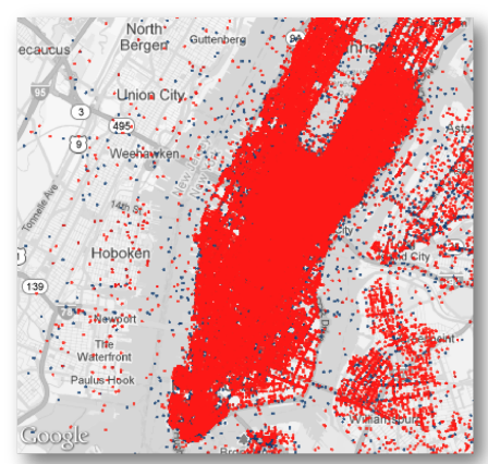
Every trip drawn as a point: Manhattan is a solid red mass

Solution 1: Adaptive Level of Detail (LOD)

Strategy: Render only what you can see

  • Sort points along a Z-order curve, build a binary tree
  • The first n elements are a hierarchical subsample of size n
  • n scales with the zoom level

Result: a readable sample at every zoom level
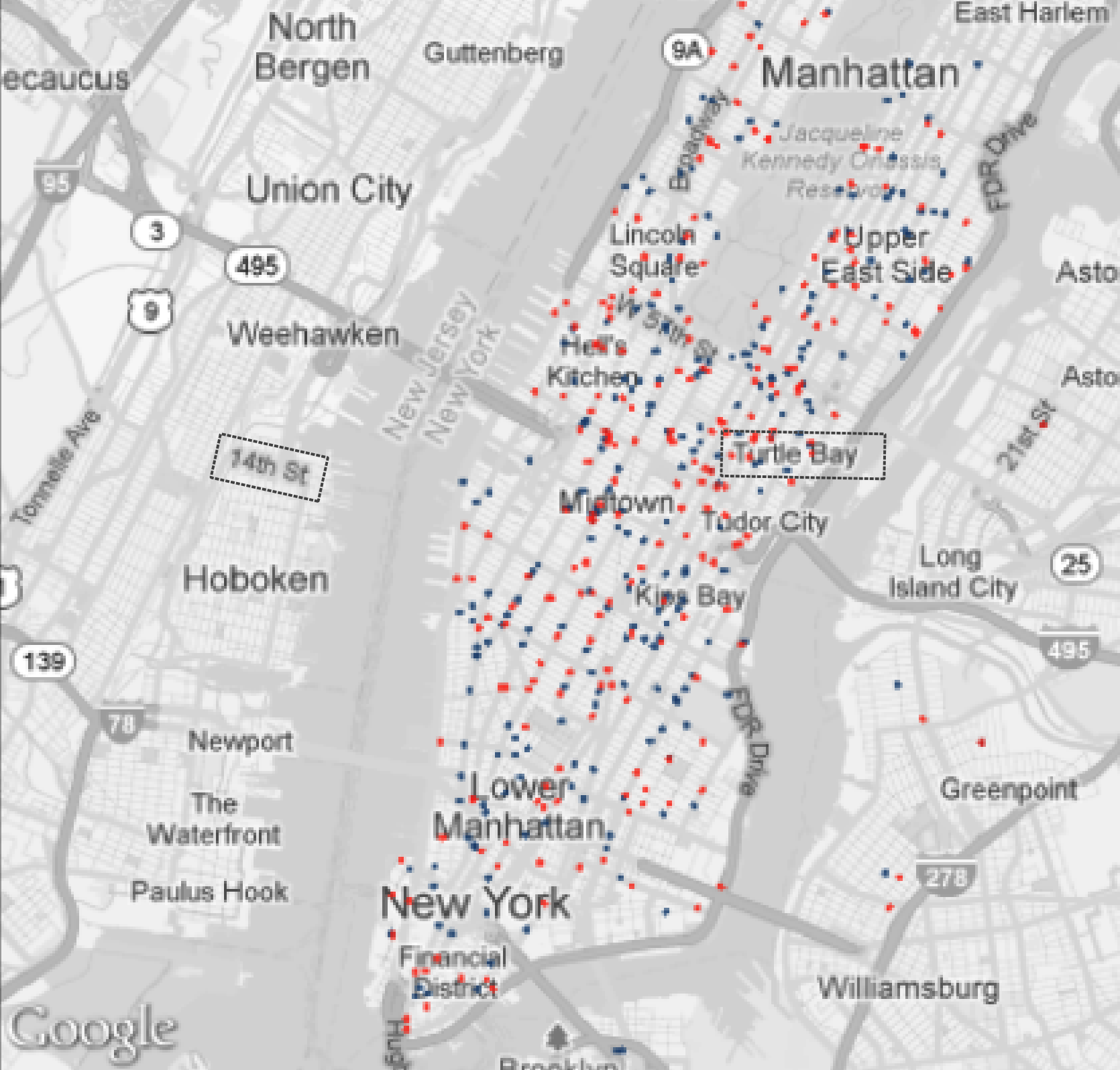
A hierarchical sample of the same trips: a readable subset instead of a blob

Solution 2: Heat Maps and Neighborhood Maps

Continuous Heat Maps
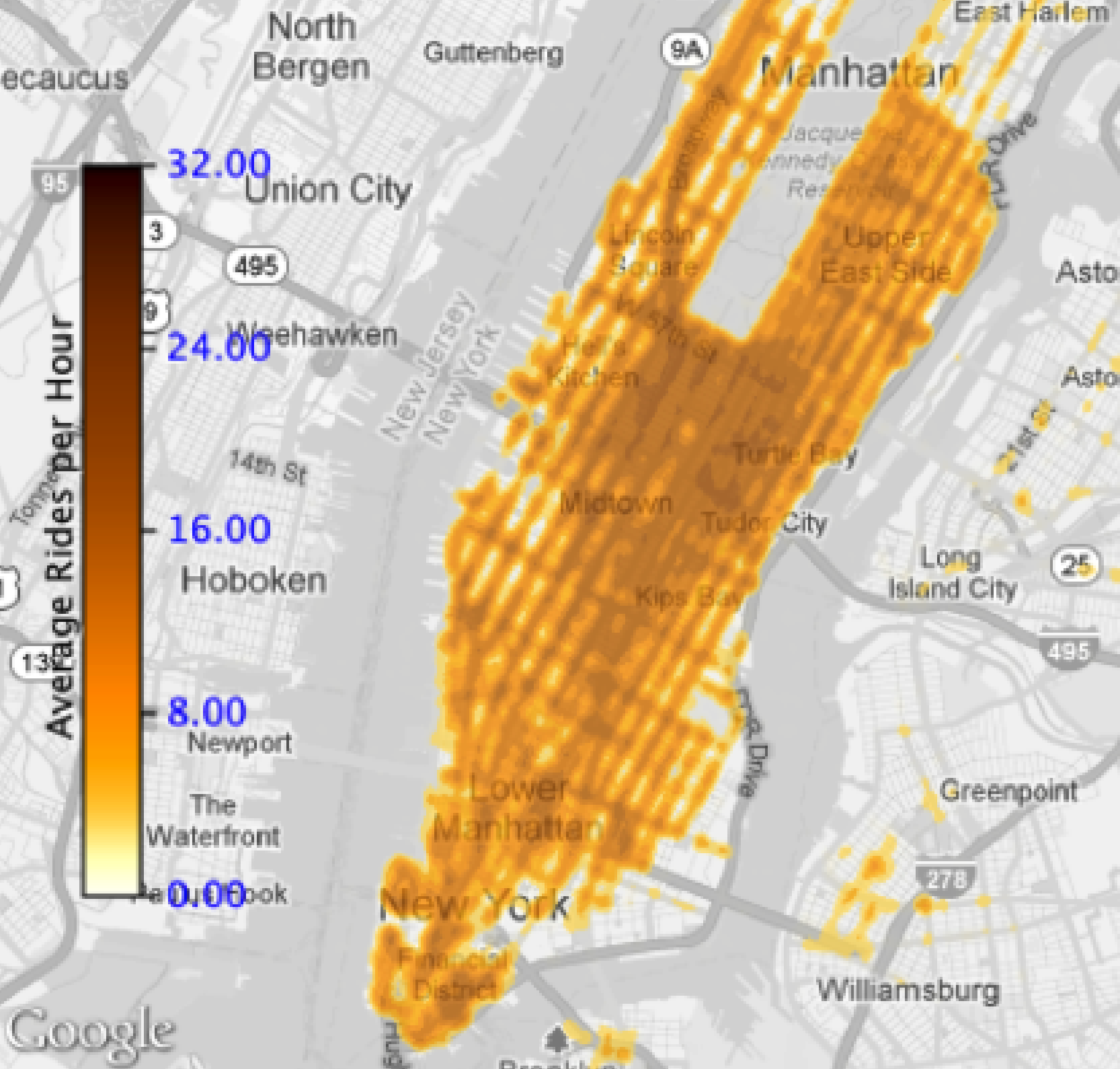
Pixel-based density heat map of Manhattan
  • Pixel-based density, darker = more activity
  • Shows the overall distribution

Neighborhood Maps
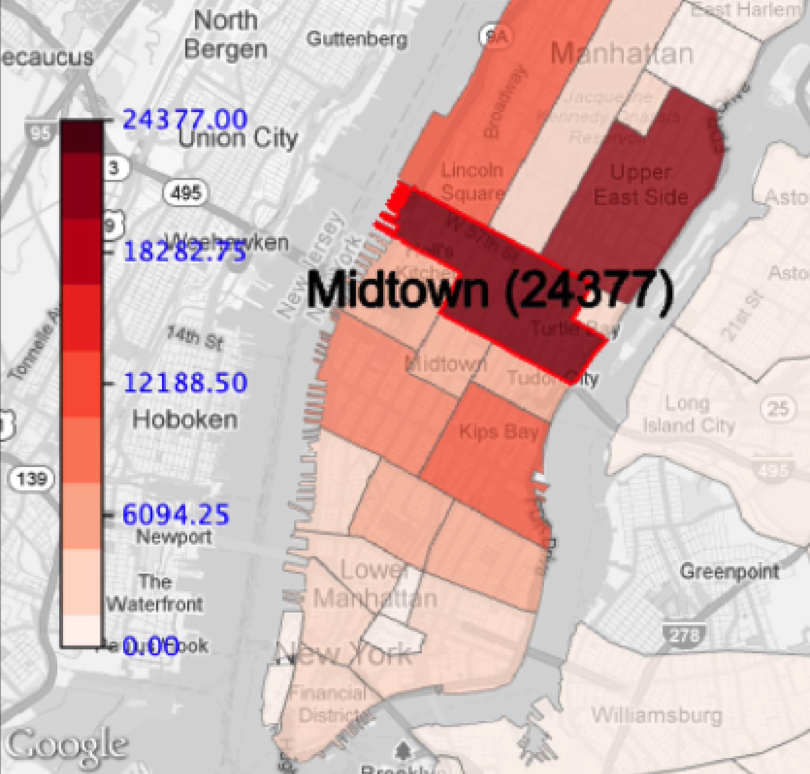
Choropleth of trips per neighborhood; Midtown selected (24,377)
  • Aggregate by meaningful regions
  • Select a region to read its exact count

When to use: heat maps for overview and patterns, LOD for individual trips, neighborhood maps for comparing defined regions

Solution 3: Multiple Coordinated Views

The Comparison Problem:

  • “How do Sundays differ from Mondays?”
  • “JFK vs. LGA patterns?”
  • “This year vs. last year?”

Solution:

  • Side-by-side views
  • Each view = one query (color-coded)
  • Synchronized spatial extent
  • Linked plots and summaries
  • Interactive refinement

Sunday (left) and Monday (right) airport queries side by side

Part 12: Linked Views & Brushing

Core Concept: Brushing and Linking

Actions in one view are reflected in all other views

This creates a “dialogue” where you can ask questions by interacting with any visualization component, and all views update to answer your question.

Example: Spatial Selection → Temporal Pattern

“What is the temporal pattern for trips from JFK Airport?”

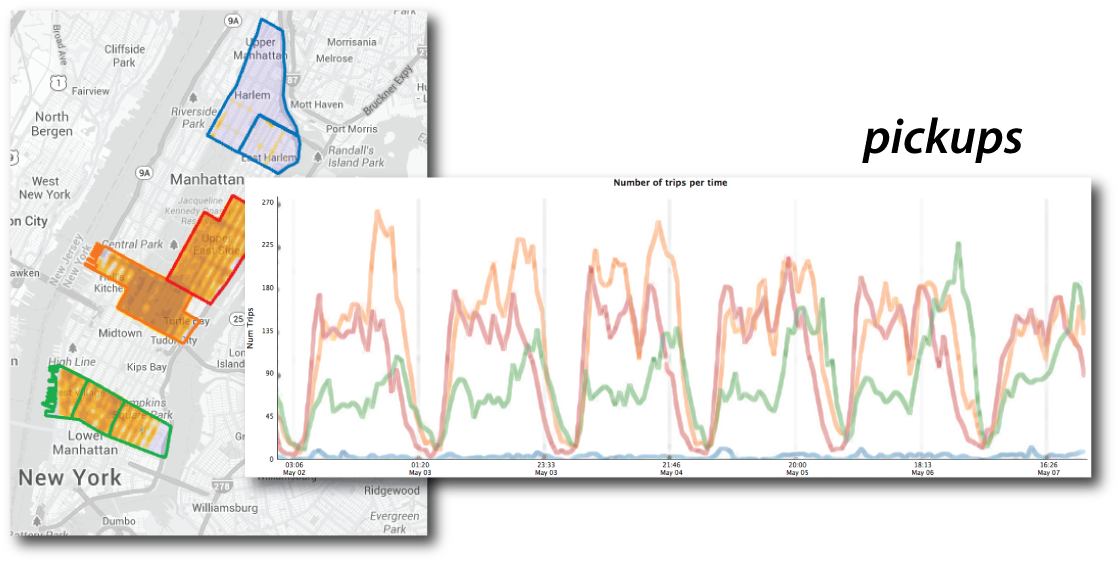
Linked Views in Action: Regions on the Map, Lines in the Chart
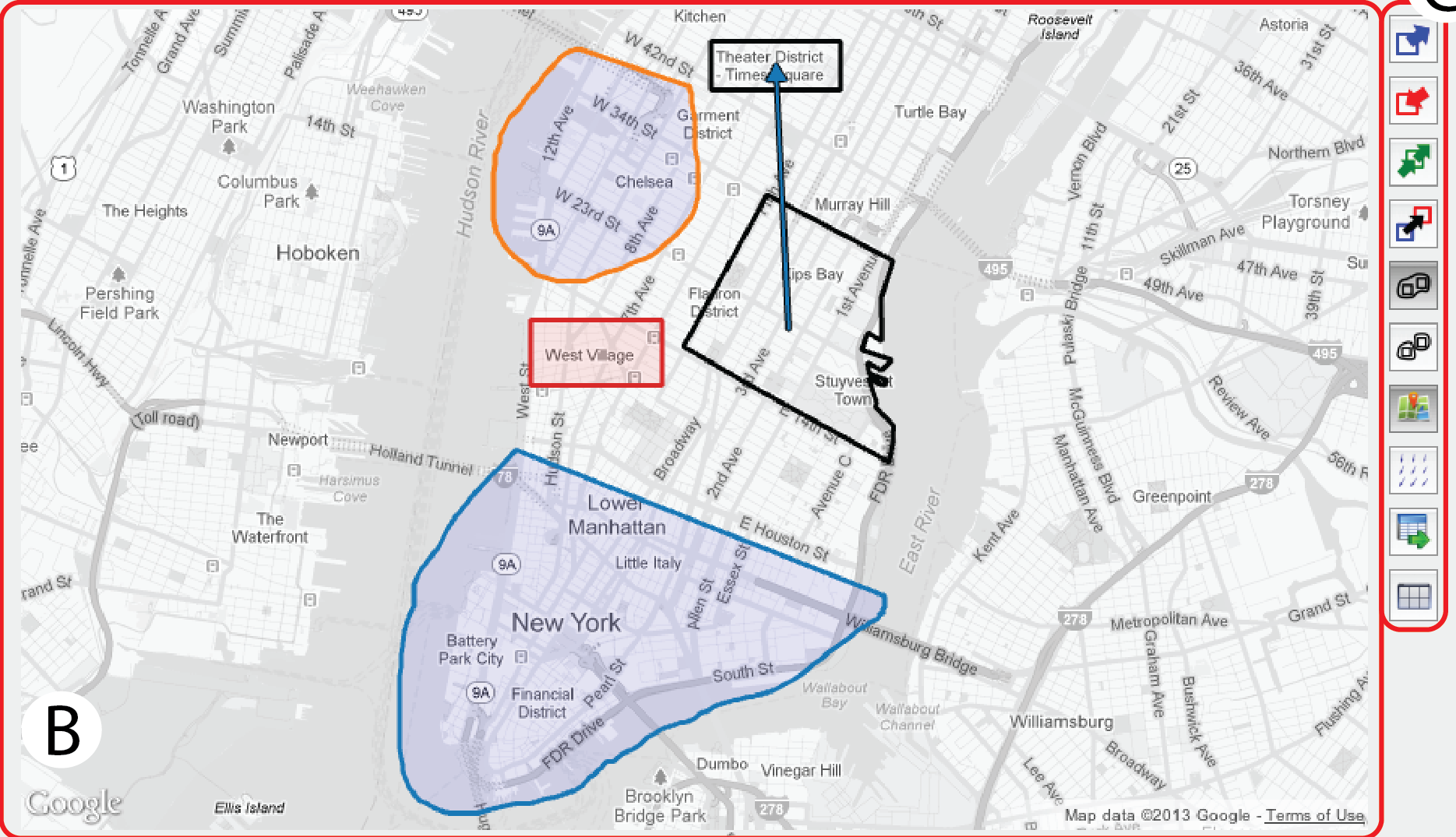
Three queries on the map

One line per query in the chart, same colors

Draw regions on the map and the chart answers: one line per query, matched by color.

The Power of Bidirectional Linking

The linking works in both directions

  • Spatial → Temporal: Select a region → see temporal patterns
  • Temporal → Spatial: Set a time window → the map shows only those trips

This bidirectional dialogue enables exploratory analysis that would be impossible with static visualizations.

Part 13: Temporal Queries

Temporal Slicing: Time → Space

The Question:

“Where are the trips in this hour of the day?”

The Interaction:

  1. Set start time, end time and step size in the time widget
  2. The map redraws with only the trips in that window
  3. Step forward or back one step at a time

The time widget: start, step size, end

TaxiVis showing one hour of trips (Sunday May 1, 2011, 12-1 AM)

Advanced Temporal Queries: Recurrent Selection

Select recurring time periods: a pattern, not a single time slice.

Recurrent selection widget: shaded years, month, weekdays and hours are the selected pattern

Shaded here: September of 2011 and 2012, Tuesdays and Fridays, 9-11 AM. Other examples: all Mondays 8-10 AM, every Saturday night, weekday rush hours only.

This reveals periodic behavior: the heartbeat of the city.

Part 15: Origin-Destination Queries

The Most Powerful Query: Flows

Asking about movement between specific locations

Traditional Approach:

SELECT * FROM trips
WHERE origin = 'JFK'
AND destination = 'LGA'
AND time BETWEEN '8:00' AND '10:00'

Complex, requires knowing SQL and field names

TaxiVis Approach:

Draw an arrow

Simple, visual, intuitive

This is what we mean by “visual query”—you draw your question, the system answers. You have already seen it: the blue and red arrows in the airport query.

Visual Queries: Why They Matter

  1. Lower cognitive load
    • No need to remember field names or syntax
    • Direct manipulation of the data representation
  2. Immediate feedback
    • See results instantly as you interact
    • Iterate quickly through hypotheses
  3. Support exploration
    • Encourages “what if” questions
    • Makes serendipitous discovery possible
  4. Democratize analysis
    • Analysts without SQL/programming skills can explore
    • Domain experts can directly investigate questions

The visualization is the interface.

Part 16: Case Study 1 - Social Inequality

Question: “Are some neighborhoods underserved by taxis?”

The Analysis:

  • Compare taxi activity across four areas: Harlem (with East Harlem), Upper East Side, Midtown, and Downtown (the Villages)
  • Pickups and dropoffs over one week in May 2011

Keep in Mind:

  • These are counts, not rates
  • Regions differ in size and population
  • What would you normalize by?

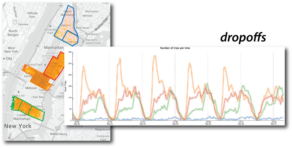
The Discovery: Over 10x Difference

Pickups: Harlem (blue) is flat next to Midtown, the Upper East Side and Downtown

Dropoffs: the same comparison

Harlem (blue) sits more than an order of magnitude below Midtown, in pickups and in dropoffs.

Follow-Up Investigation

The exploration followed a natural path:

  1. Initial pattern: Harlem has far fewer taxi trips
  2. Hypothesis: Is this an economic issue?
  3. Investigation 1: “Are tips different in Harlem?”
    • Discovery: Tips per trip are higher (and noisy: few trips)
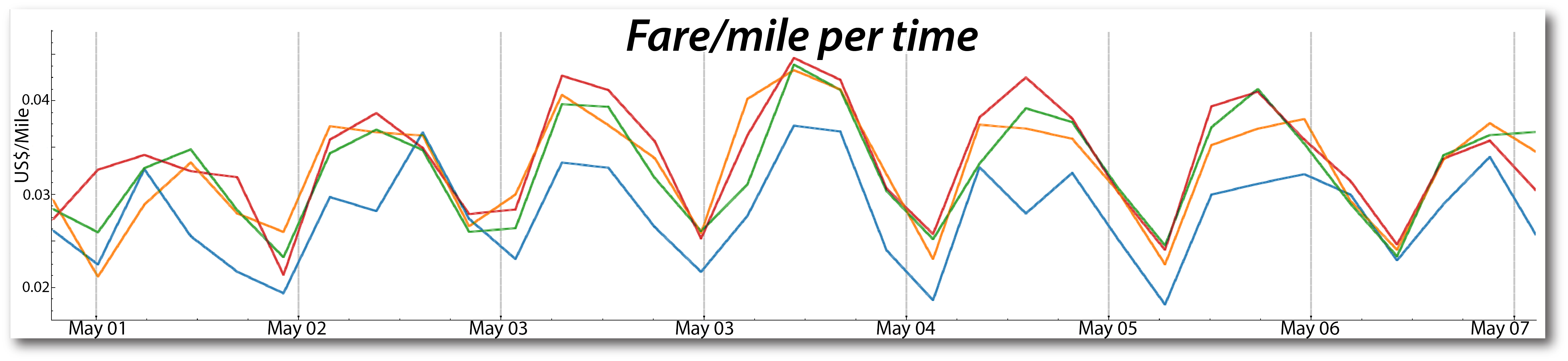
  4. Investigation 2: “Is fare per mile different?”
    • Discovery: Consistently lower fare per mile
  5. Insight: Less economic incentive for taxis to be in Harlem; the higher tips may be a way to reward drivers who go

Follow-Up Investigation: The Two Charts
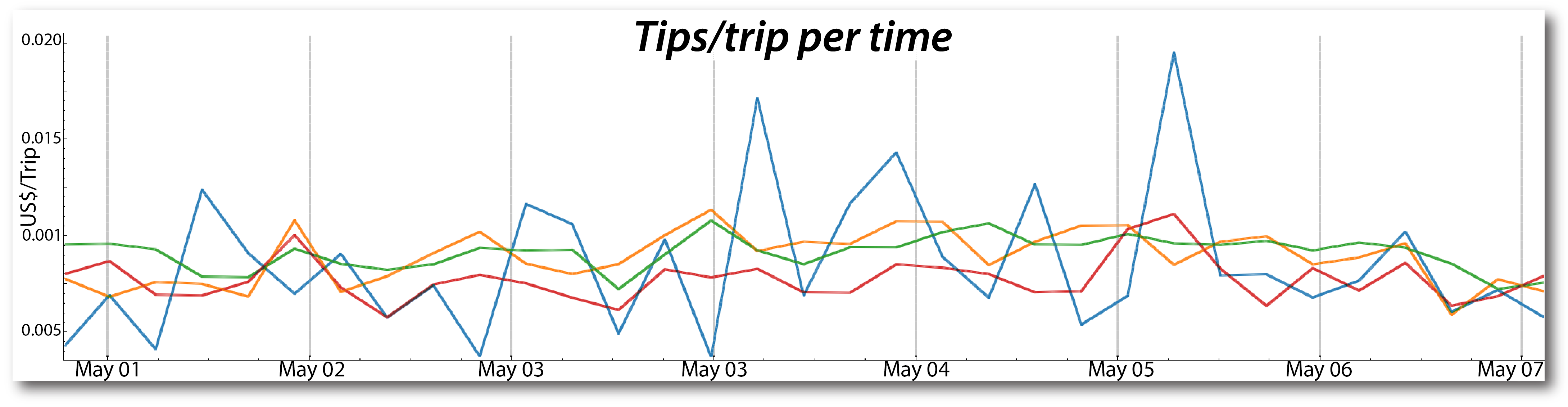
Blue = Harlem. Tips per trip run higher but noisily (few trips); fare per mile is lower.

Part 17: Case Study 2 - Transportation Hubs

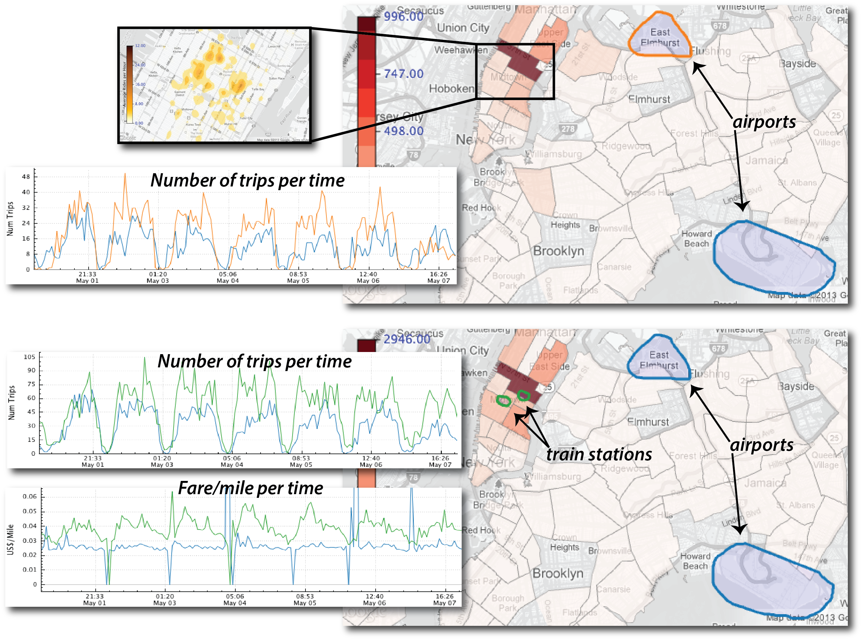
Question: “How do people move through NYC’s transportation infrastructure?”

The Setup:

  • Compare JFK, LGA, Penn Station, Grand Central
  • Use grouping to combine regions
  • Examine pickup patterns over one week

Airports vs. train stations: trips per time (top) and fare per mile (bottom)

Key Findings

  1. More pickups at LGA than JFK on most days

  2. Train stations >> airports for pickups

  3. Weekday pattern: train-station pickups roughly constant Mon-Thu, falling Friday to a low on Saturday

    • Reflects commuter behavior
  4. Rush hour problem: airport trips take much longer around 3-5 PM; fare per mile is higher within Manhattan

    • Economic incentive to avoid airport trips
    • Refusing rides is illegal, but a common practice for JFK

Part 18: Case Study 3 - Temporal Exploration

Time-Space Exploration

Feature:

  • Select multiple time slices automatically
  • Compare the same time across days, weeks or months
  • Each slice gets its own map and its own colored line

Example: Memorial Day Analysis

  • All Mondays in May 2011 and May 2012
  • Nine maps, nine lines

Discovery: Memorial Day Pattern

Maps for each Monday (a) and one line per Monday (b): two lines stand apart.
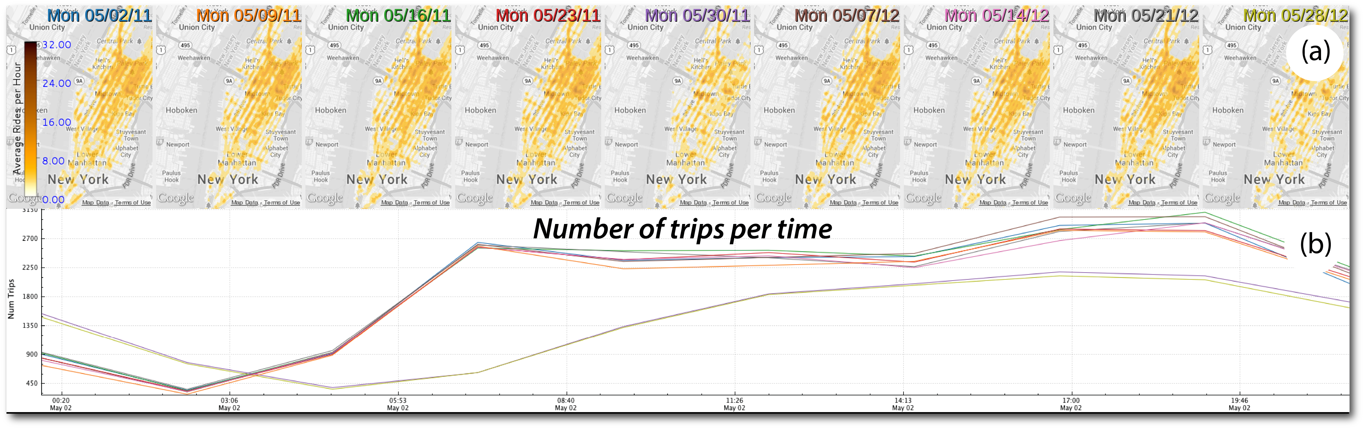
Nine May Mondays: maps (a) and trips per time (b)

  • Discovery: Memorial Day (May 30, 2011 and May 28, 2012) has significantly fewer trips than the other Mondays
  • Implication: Fleet size could be reduced on holidays to save costs

Part 19: Case Study 4 - Hurricane Sandy

Question: “How did Hurricane Sandy affect NYC?”

The Analysis:

  • One week of taxi activity
  • Sunday before through Saturday after
  • Heat maps for each day
  • Compare spatial patterns

The Timeline:

  • Sunday (before): Normal activity
  • Monday (hurricane hits): Virtually no taxis citywide
  • Tuesday-Friday: Activity returns everywhere EXCEPT Lower Manhattan
  • Saturday: Finally returns to normal

The Story the Data Tells

Daily heat maps of taxi pickups, Sunday Oct 28 to Saturday Nov 3, 2012

Why? Lower Manhattan had a multi-day power outage. You can see it on the map.

Comparison to Hurricane Irene
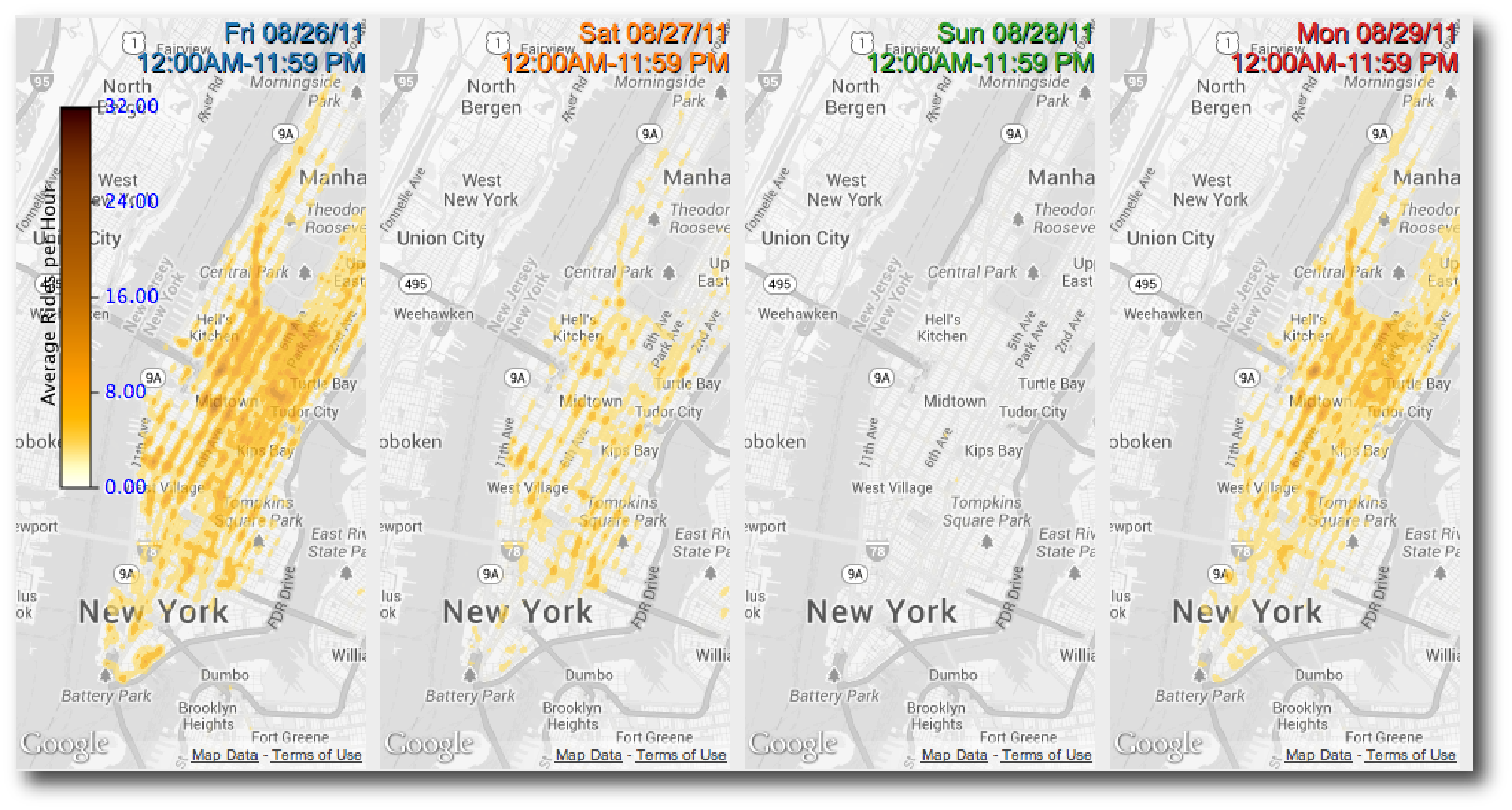
Irene: daily heat maps for Fri Aug 26 to Mon Aug 29, 2011
  • Shorter disruption but more complete
  • Only 1,076 trips on the hurricane day (vs. an average of about 500,000)
  • Faster recovery

Part 20: What We Learned

Design Insights from Building TaxiVis

  1. Visual queries work
    • Early users found it usable without SQL or programming
    • No SQL, no programming required
  2. Performance is non-negotiable
    • Sub-second response enables exploration
    • Adaptive rendering essential for large results
  3. Multiple views are essential
    • Comparison is core to analysis
    • Side-by-side queries, synchronized views
    • Linked plots and maps
  4. Query composition is powerful
    • Build complex queries from simple ones
    • Grouping, refinement, generalization

Part 21: Real-World Impact

Who’s Using TaxiVis?

Users:

  • Designed from interviews with 5 NYU researchers: 2 traffic engineers and 3 economists
  • Deployed to a few domain scientists at NYU
  • Data provided by the NYC Taxi & Limousine Commission
  • Feedback “very positive”; larger usability study planned

What They’ve Learned:

  • Social inequalities in taxi service (Harlem)
  • Economic incentives affecting driver behavior
  • Impact of major events on city mobility
  • Transportation hub usage patterns

Beyond Taxis:

  • Model applies to other origin-destination data
  • Generalizes to other spatio-temporal datasets
  • Principles useful for any urban data exploration

Part 22: Key Takeaways

The Big Ideas

  1. Urban data is fundamentally spatio-temporal
    • Space, time, and attributes all matter
    • Need to explore interactions, not just individual dimensions
  2. Static visualization is not enough
    • Interactivity transforms presentation into exploration
    • “Dialogue with data” through visual queries
  3. Design for domain experts, not data scientists
    • Visual operations instead of code
    • Direct manipulation over programming
    • But don’t sacrifice expressiveness
  4. Performance enables exploration
    • Sub-second response changes how people think
    • Specialized systems beat general solutions
    • Trade generality for interactivity

Part 23: From TaxiVis to Urban Analytics

The Broader Vision

TaxiVis is One Example

Other urban data:

  • Bikeshare systems
  • 311 service calls
  • Building permits
  • Transit ridership
  • Crime reports
  • Traffic sensors

Same challenges: Scale, complexity, spatio-temporal nature

The Visual Analytics Framework

  1. Visualization: Multiple representations and query models
  2. Data Analysis: Topology, ML, pattern detection
  3. Data Management: Specialized indices, GPU acceleration

Moving to 3D

Cities are vertical, not just horizontal

  • Shadow analysis
  • Views and sight lines
  • Sky exposure
  • Building massing

Next Lecture:

We’ll extend these ideas to 3D urban visualization and the Urbane framework

Same principles apply: interactive, visual, scalable

Summary

The Visual Analytics Pipeline for Urban Data

What We’ve Covered Today:

The Problem:

  • Urban data is big, complex, spatio-temporal
  • Traditional tools don’t scale
  • Confirmation vs. exploration gap

The Solution:

  • Visual query models for direct manipulation
  • Interactive performance through specialized systems
  • Multiple visualizations for different questions
  • Comparison through coordinated views

The Result:

  • Domain experts can explore without programming
  • Discoveries about social inequality, economics, events
  • Real impact on city operations and policy

Try It Yourself - Exploration Exercise

If you had access to TaxiVis, what would you explore?

Think about:

  • A neighborhood you’re curious about
  • A time pattern (weekday vs. weekend, holidays, events)
  • A comparison (this year vs. last year, two locations)
  • A hypothesis about urban behavior

Discussion:

  • What question would you ask?
  • What spatial regions would you select?
  • What time slices would you compare?
  • What would you expect to find?

Optional: Build Your Own with Autark

Autark (autark.js): urban visual analytics in the browser

  • Website: autarkjs.org (MIT license)
  • Install: npm install @urban-toolkit/autk
  • Serverless: load, process and visualize geospatial data entirely client-side
  • autk-db: geospatial queries on OpenStreetMap, GeoJSON, GeoTIFF and CSV
  • autk-map: 2D and 3D maps rendered with WebGPU
  • autk-plot: interactive D3 charts linked to the map
  • autk-compute: custom analysis on GeoJSON

How it connects to today

  • Map + linked charts = the brushing and linking idea, now something you can build
  • The gallery already has linked views, and GPU analyses (sky exposure, visibility, view score) that preview next week’s 3D class
  • Start with the Observable tutorial or the gallery
  • Optional; a good fit if your mini-project uses urban data
  • Maps and GPU analyses need WebGPU: Chrome or Edge 113+, Safari 26+, Firefox 141+

Optional: Try TaxiVis Yourself

The revamped TaxiVis is open source

  • Repository: github.com/vida-nyu/taxivis
  • A desktop application (C++, Qt 6, OpenGL), not a web page
  • Build from source with CMake; instructions for macOS (Homebrew) and Ubuntu are in the README
  • Same ideas as today: draw regions and arrows on the map, set time windows, linked time series, histograms, scatter plots and heat maps

What to expect

  • A small sample of 10,000 trips is bundled, enough to check the build
  • To explore for real, you prepare a month of NYC TLC trip data (about 14-15 million trips) with the README’s pipeline
  • Entirely optional, and it takes some setup time
  • The screenshots in today’s lecture are from the 2013 version, so the new interface will look different

This Week

  • Mini-Project 2 begins: Temporal visualization (due Nov 19)
  • Exercise 9: Urban data exploration and visual queries (due Nov 5)
  • Reading: Ferreira et al. (2013), Visual Exploration of Big Spatio-Temporal Urban Data, IEEE TVCG
  • Lab: building interactive spatio-temporal visualizations in D3
  • Optional: try the revamped TaxiVis (build from source)
  • Optional: explore Autark, our browser-based urban analytics toolkit

Questions?

Next week: 3D & Immersive Urban Visualization

Preview:

  • Urbane framework for 3D urban planning
  • Interactive impact analysis (shadows, views, sky exposure)
  • Performance-driven architectural design
  • When to use 3D (and when not to)