VisML Lab: Deep Learning, Hands-On

DS-GA 3001 - Fall 2026 - Playing with Neural Networks

Claudio Silva

NYU Center for Data Science

2026-10-27

Lab Overview

• Today: make tonight’s lecture concrete by breaking and fixing small neural networks
• Two browser tools, no installs: TensorFlow Playground and CNN Explainer
• Work in pairs. For each experiment, predict first, then test
• Next week: Visualization for NLP and LLMs

This lab is run by Claudio directly. Every experiment follows the same loop: state a prediction out loud, run it, and explain any surprise. The point is to connect the lecture’s ideas (linear vs non-linear, learning rate, depth) to what a visualization shows you.

Plan for tonight (50 minutes)

	Minutes
Tour of the Playground	5
Experiments 1-4 in the Playground	25
CNN Explainer	12
Debrief	8

Experiments 3 and 4 are optional if we run short.

The Playground in One Slide

• Data: four 2-D datasets (circle, XOR, Gaussian, spiral)
• Features: what the network gets to see: \(x_1\), \(x_2\), and hand-made combinations
• Hidden layers: add or remove layers and neurons with the + / − buttons
• Output: the decision boundary, with training and test loss

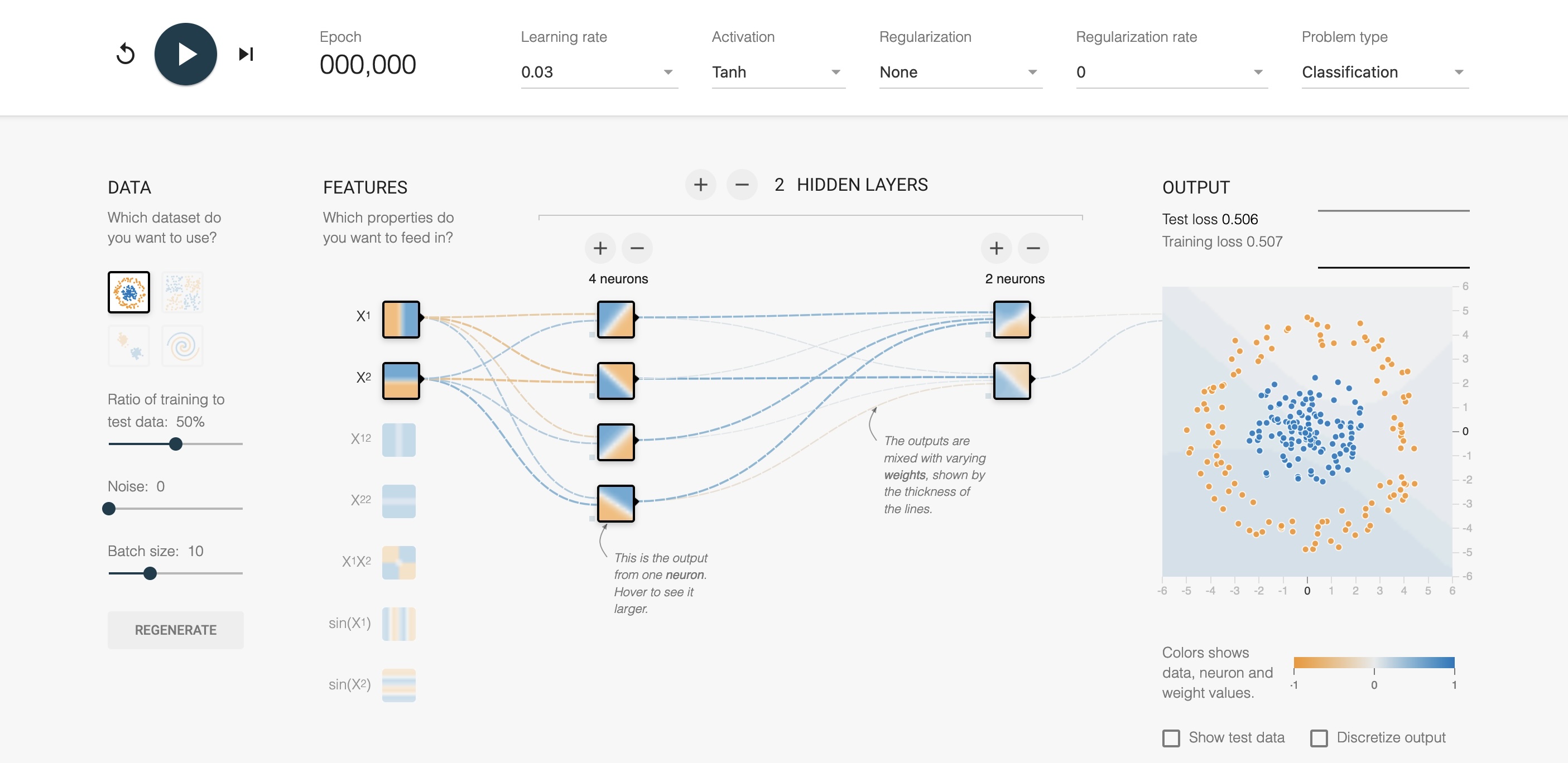
Open https://playground.tensorflow.org now. Press play once to see training run.

Experiment 1: Why Do We Need Hidden Layers?

Predict: can a network with no hidden layers separate the circle dataset?

1. Choose the circle dataset. Features: only \(x_1\) and \(x_2\). Remove all hidden layers. Train.
2. Add one hidden layer with 4 neurons (activation: tanh). Train again.
3. Hover over each hidden neuron. What shape does each one draw?

Connect to lecture: a linear model gives a straight boundary; hidden units are the “bent lines” we composed.

Expected result: no hidden layers can only draw a straight line, so the circle stays unsolved and loss stays high. With one hidden layer of a few neurons the boundary closes into a blob around the inner class. Each hidden neuron shows a simple, roughly linear boundary; the output layer combines them. This is the “composing ReLUs / bent lines” slide made visible.

Experiment 2: What Does the Activation Do?

Predict: what happens if the activation is linear and we add more layers?

1. Use the circle dataset with a 2-layer network (4 + 2 neurons). Set the activation to Linear. Train.
2. Switch to ReLU, then Tanh. Compare the boundaries.
3. Return to Linear and make the network much bigger. Does the boundary change character?

Connect to lecture: without a non-linear activation, composing layers is still one linear function.

Expected result: with a linear activation the boundary stays a straight line no matter how many layers or neurons. ReLU gives piecewise-linear (angular) boundaries; tanh gives smoother ones. This is why activation functions were the key step in the “From Linear to Non-linear” slide.

Experiment 3: Learning Rate

Predict: what happens at learning rates 0.003, 0.03 and 3?

1. Use the circle dataset, 1 hidden layer of 4 neurons, Tanh. Reset between runs.
2. Run each learning rate for the same number of epochs. Watch the loss curve (top right of the output panel).
3. Which rate converges fastest? Which one is unstable?

Connect to lecture: \(\Phi_{new} = \Phi_{old} - \alpha \nabla L[\Phi]\). Too small is slow; too large overshoots.

Expect a slow, steady decrease at the smallest rate, a good decrease at the middle rate, and noisy, jumpy, or non-improving loss at the largest rate. Exact behavior depends on random initialization, so rerun if a run looks odd. Optional.

Experiment 4: The Spiral

Predict: how small can the network be and still solve the spiral dataset?

1. Start with only \(x_1\), \(x_2\) and one hidden layer. Train for a while.
2. Add layers and neurons until the spiral is solved. Record the smallest network you find.
3. Now go back to a small network and instead turn on extra features (\(\sin x_1\), \(\sin x_2\), \(x_1 x_2\)). Does that help?

Discuss: depth vs. width vs. better features. Which gave the most for the fewest parameters?

Results vary with random initialization, and the spiral can need many hundreds of epochs, so ask students to compare notes rather than expect one answer. Typical finding: one narrow layer struggles, a few layers of 6-8 neurons succeed, and hand-made features can substitute for depth. Ties to “Why go deep?” and the universal approximation caveats. Optional.

CNN Explainer: Setup

Open https://poloclub.github.io/cnn-explainer/

• The model is a small CNN trained on 10 image classes
• The overview shows the whole pipeline: input → convolution → ReLU → pooling → output
• Click a layer to expand it. Hover over an output cell to see which input patch produced it

Find: which layers are convolutions, which are ReLU, which are pooling?

CNN Explainer: Questions

Convolution

• Click a convolution layer, then a single activation map. What does that filter respond to?
• Do the first-layer maps look different from later-layer maps?
• How does the kernel slide across the input?

ReLU, pooling, output

• After ReLU, which pixels become exactly zero?
• What does pooling throw away? What does it keep?
• Which class gets the highest score for the sample image, and how confident is the network?

Connect to lecture: early layers = low-level features; later layers = parts and objects.

Debrief

• Which prediction did you get wrong? What did the visualization show that you did not expect?
• What can these tools not show? (Think: real data with thousands of dimensions, millions of weights.)
• Where would you need a different visualization for your project’s model?

Use this to bridge to the project proposals and to next week: language models have far too many parameters for a Playground-style view, which is why NLP and LLM visualization needs different techniques.

Further Exploration

• TensorFlow Playground and its source
• CNN Explainer
• Prince, Understanding Deep Learning, Chapters 2-4 and the accompanying notebooks
• Next week (Nov 3): Visualization for NLP and LLMs