Clustering and Dimensionality Reduction
DS-GA 3001 - Fall 2026
2026-10-13
Clustering
Etienne Bernard: “… the goal of clustering is to separate a set of examples into groups called clusters”
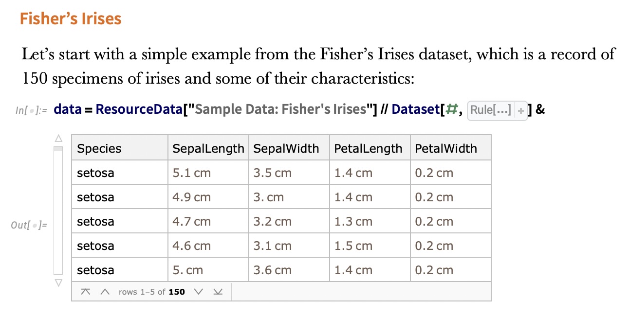
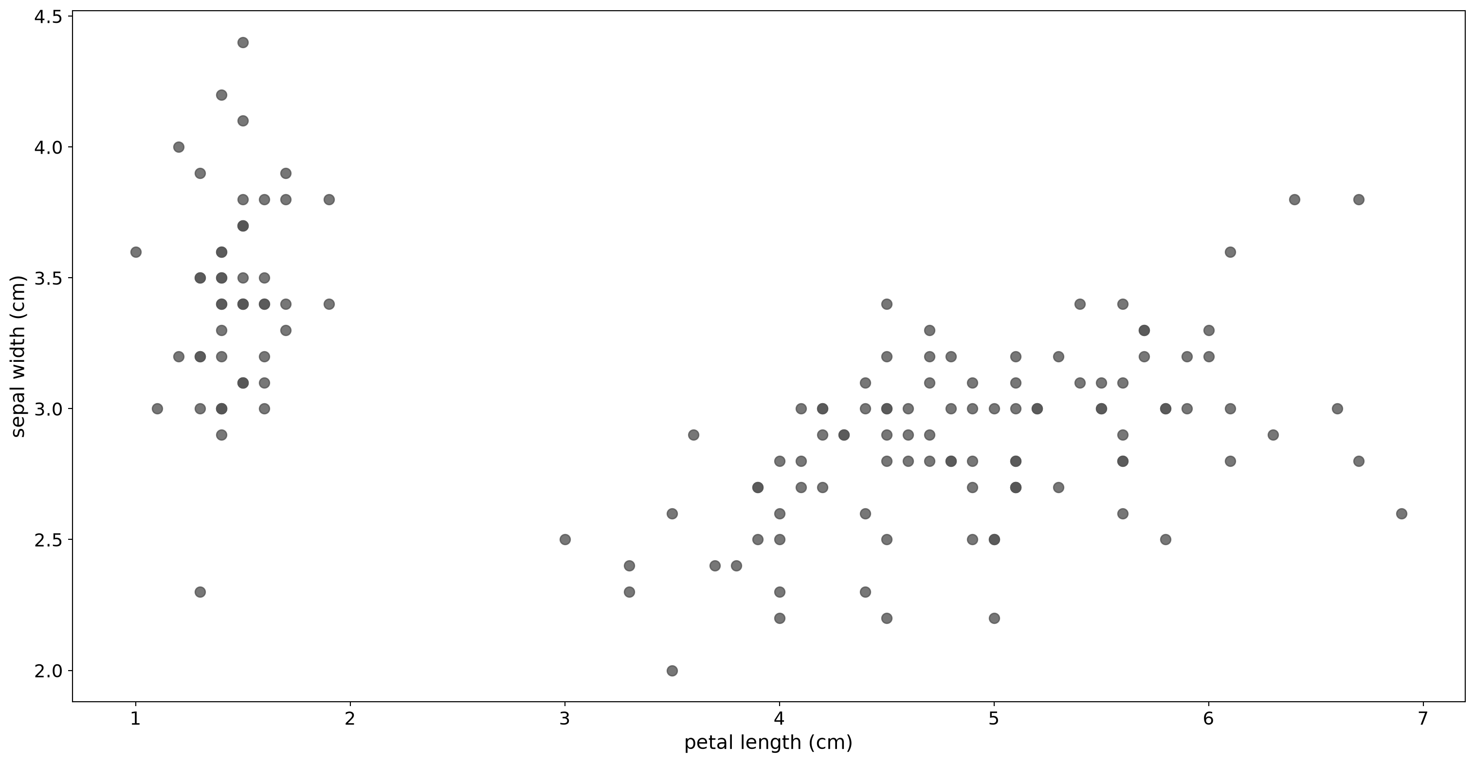
IRIS – another look
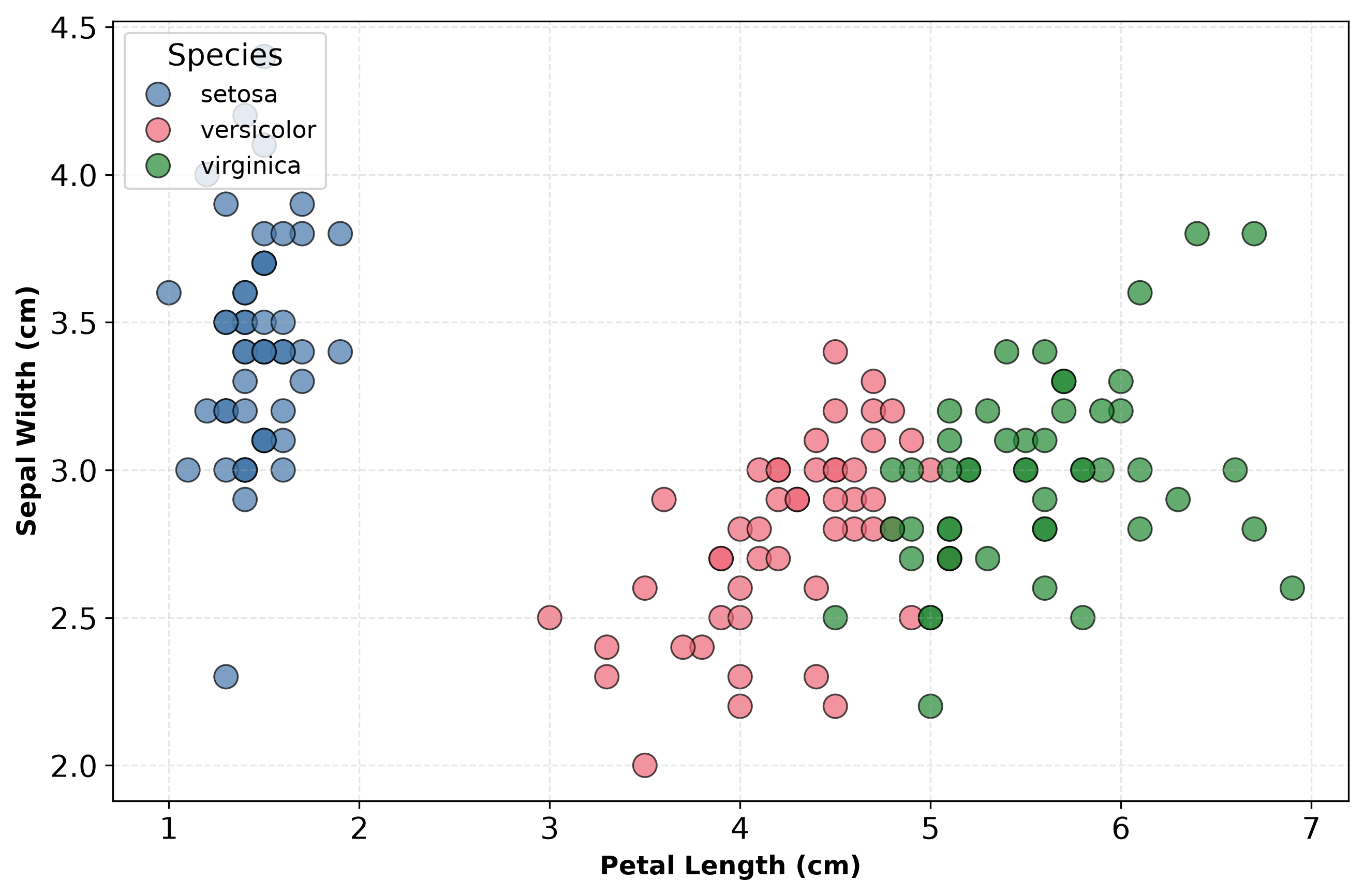
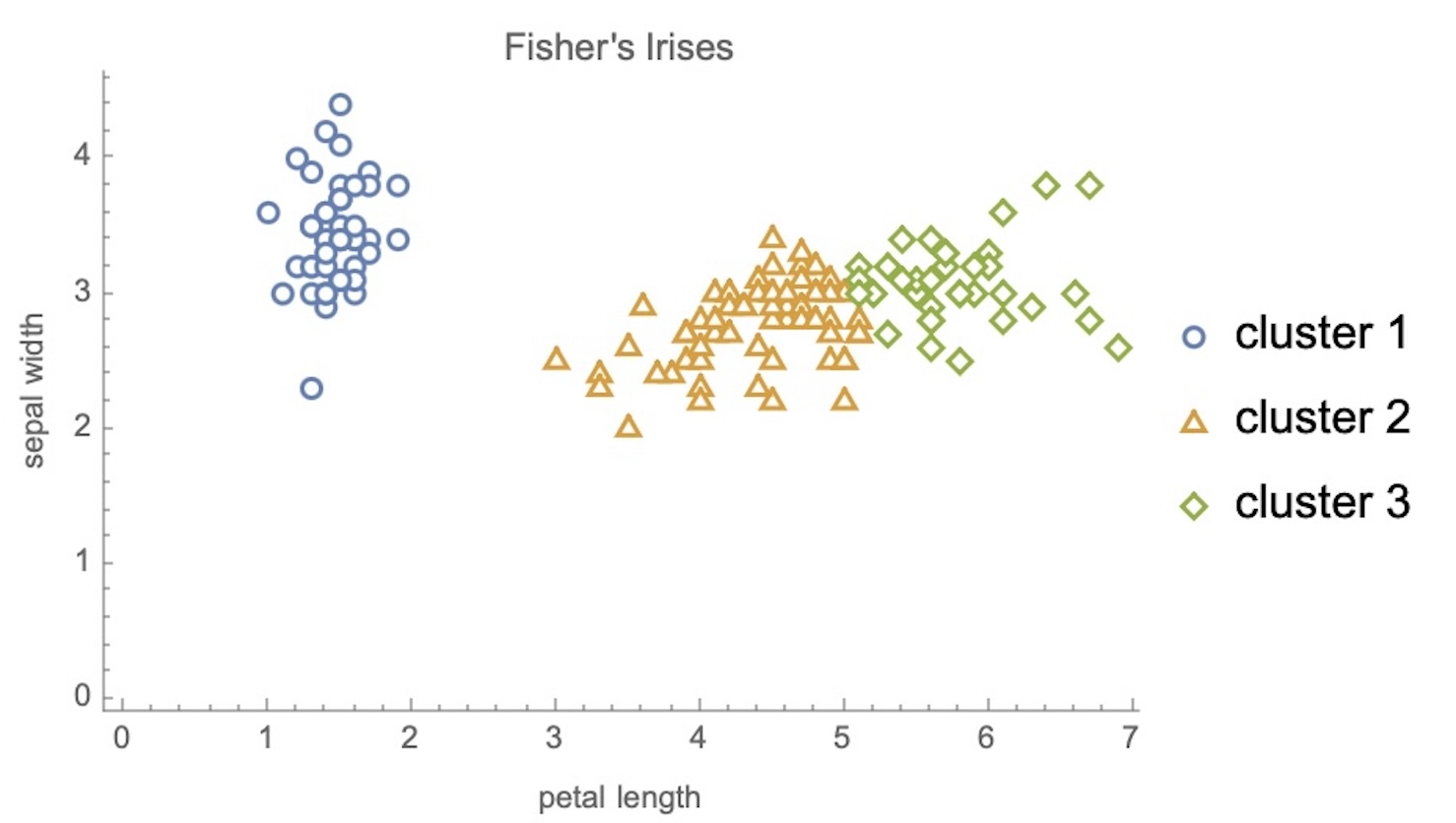
IRIS – clustering
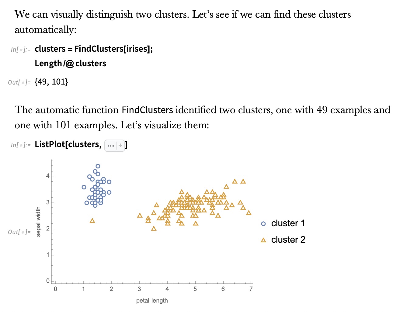
IRIS – k-means
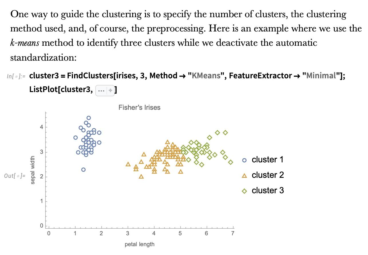
Wolfram Mathematica FindClusters
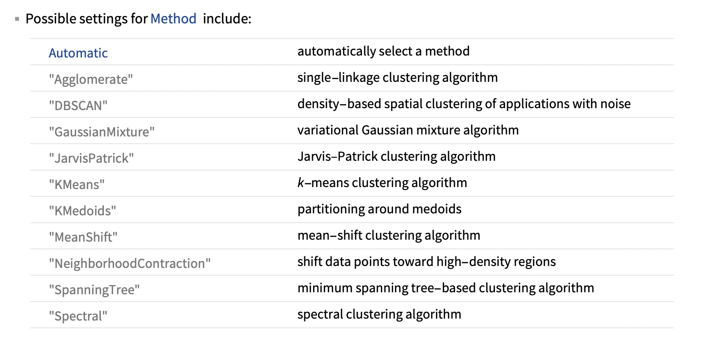
Wolfram Mathematica FindClusters
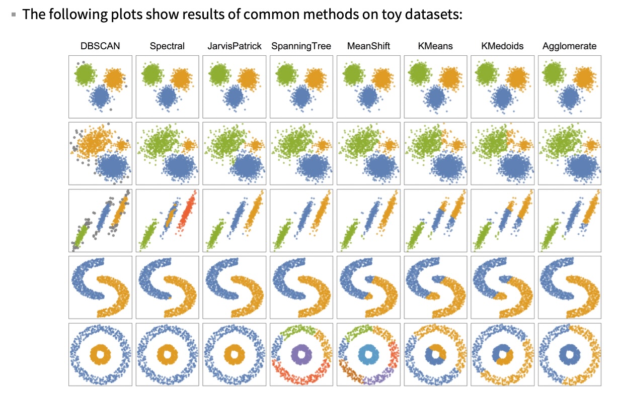
When k-means fails: shape, not count
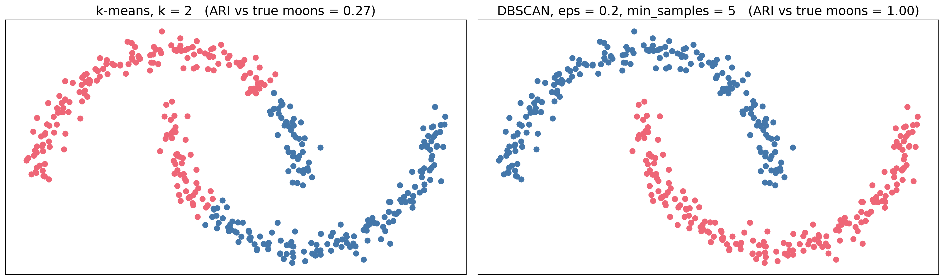
Right number of clusters, wrong definition of a cluster.
IRIS - classes
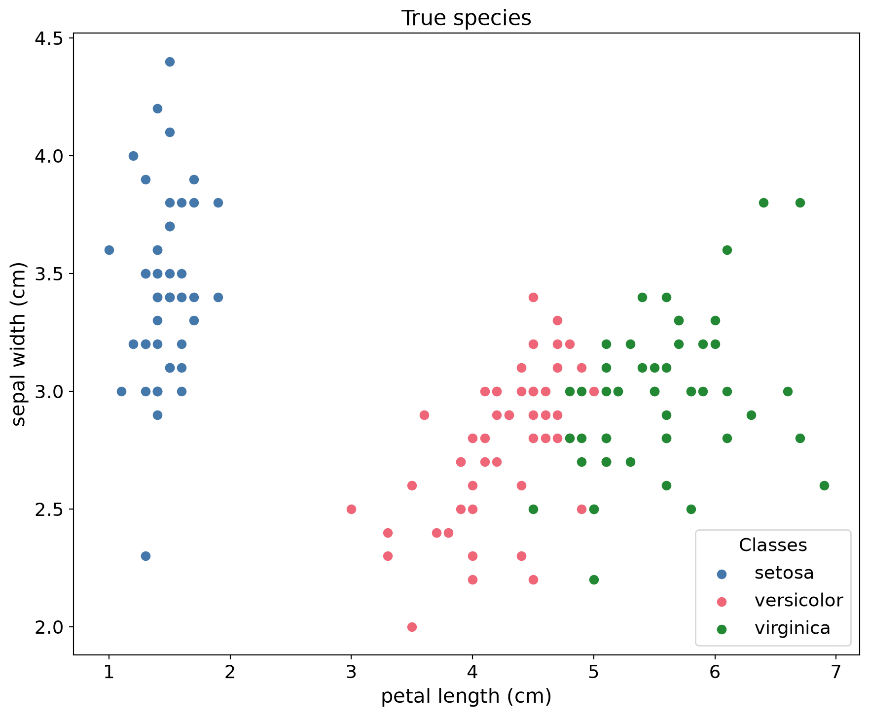
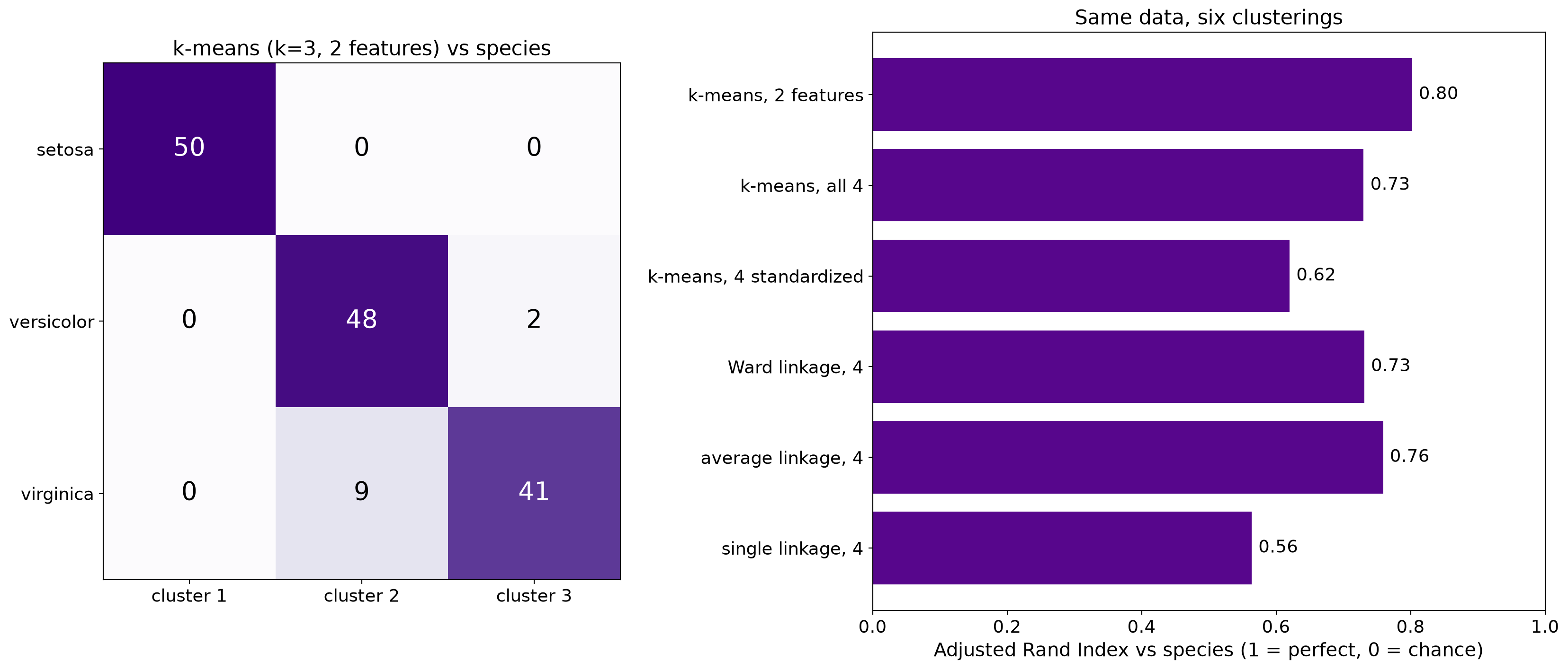
Validating clusters against labels
How many clusters? Two criteria, two answers
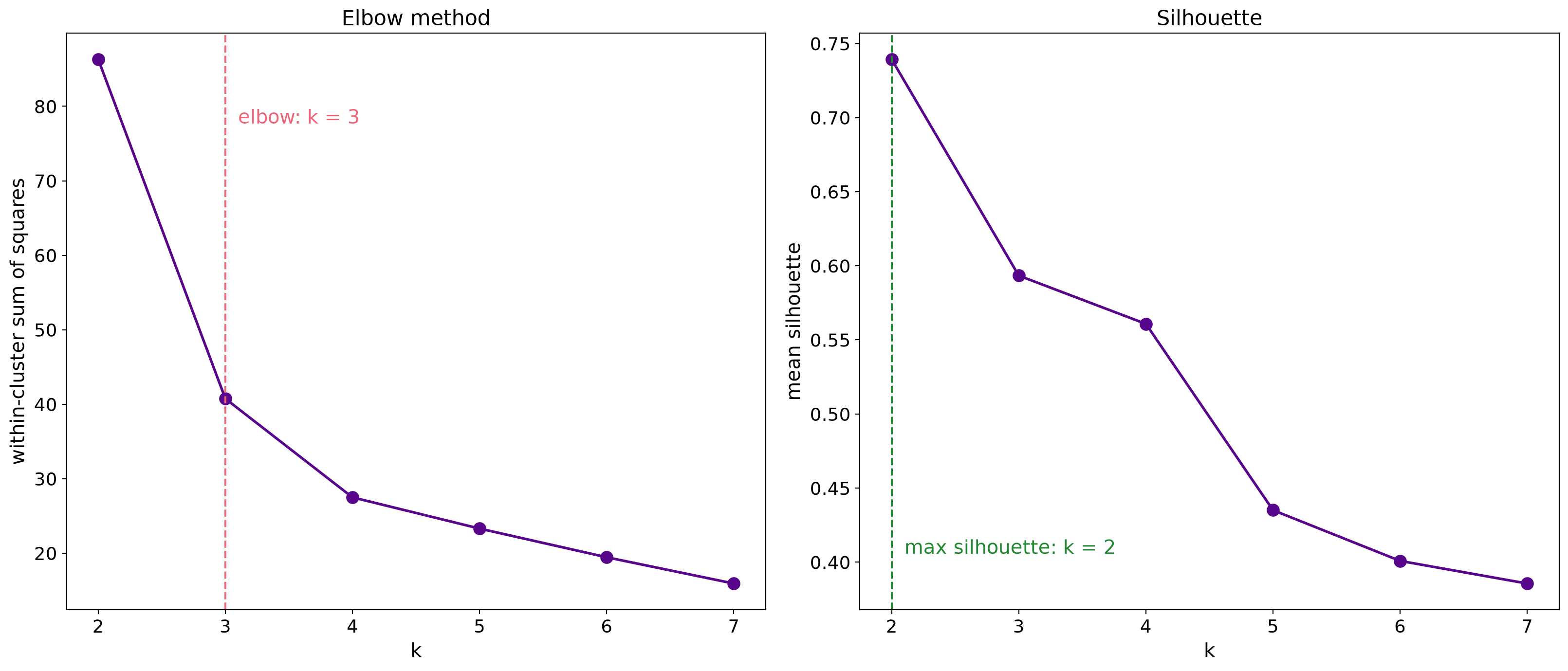
The elbow says 3, the silhouette says 2, the botanist says 3.
Hierarchical clustering: the dendrogram
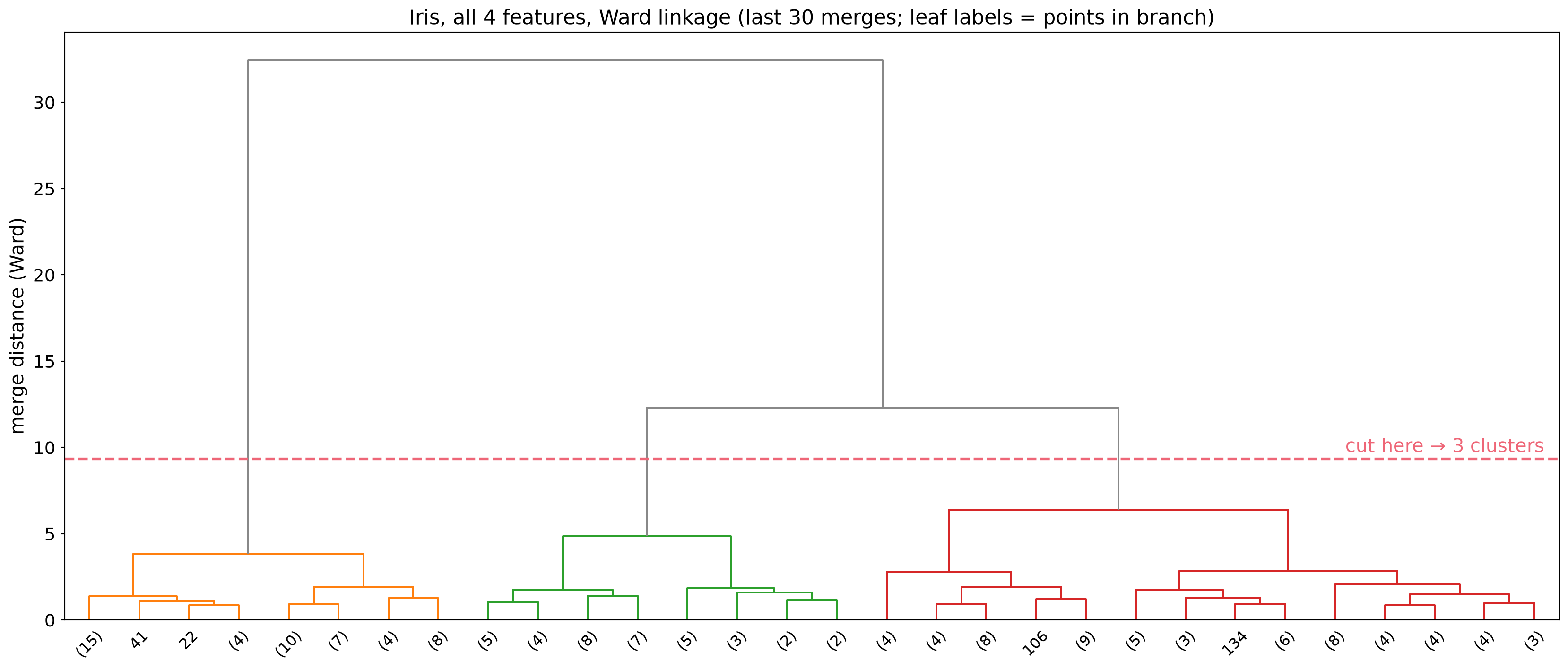
One tree, every k: the cut height is the choice.
Dimensionality Reduction
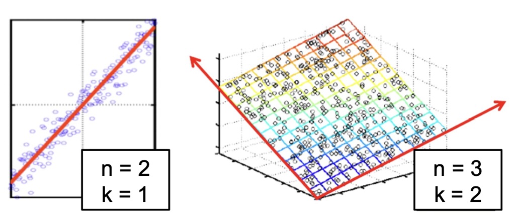
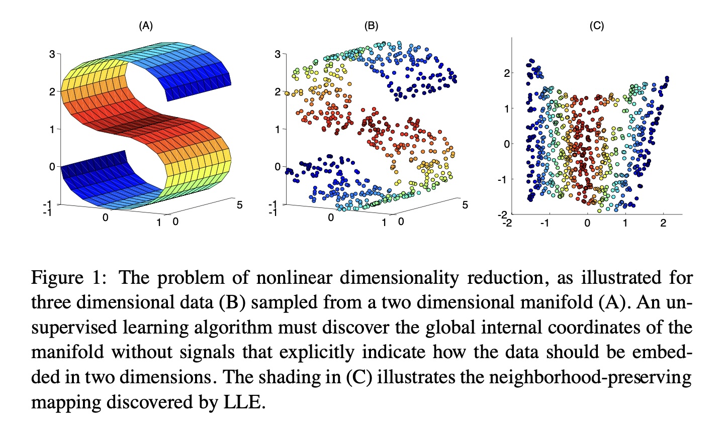
Assumption: data lies on a lower dimensional space
Visualizing the Manifold Hypothesis: Images of ‘3’ Perturbed by Non-linear Operations

What operations did we perform? What’s the intrinsic dimensionality?
Here the underlying manifold is non-linear
Digits
from sklearn.datasets import load_digits

digits = load_digits(n_class=6)
X, y = digits.data, digits.target
n_samples, n_features = X.shape
n_neighbors = 30
import matplotlib.pyplot as plt
fig, axs = plt.subplots(nrows=10, ncols=10, figsize=(8, 8))
for idx, ax in enumerate(axs.ravel()):
ax.imshow(X[idx].reshape((8, 8)), cmap=plt.cm.binary)
ax.axis("off")
_ = fig.suptitle("A selection from the 64-dimensional digits dataset", fontsize=16)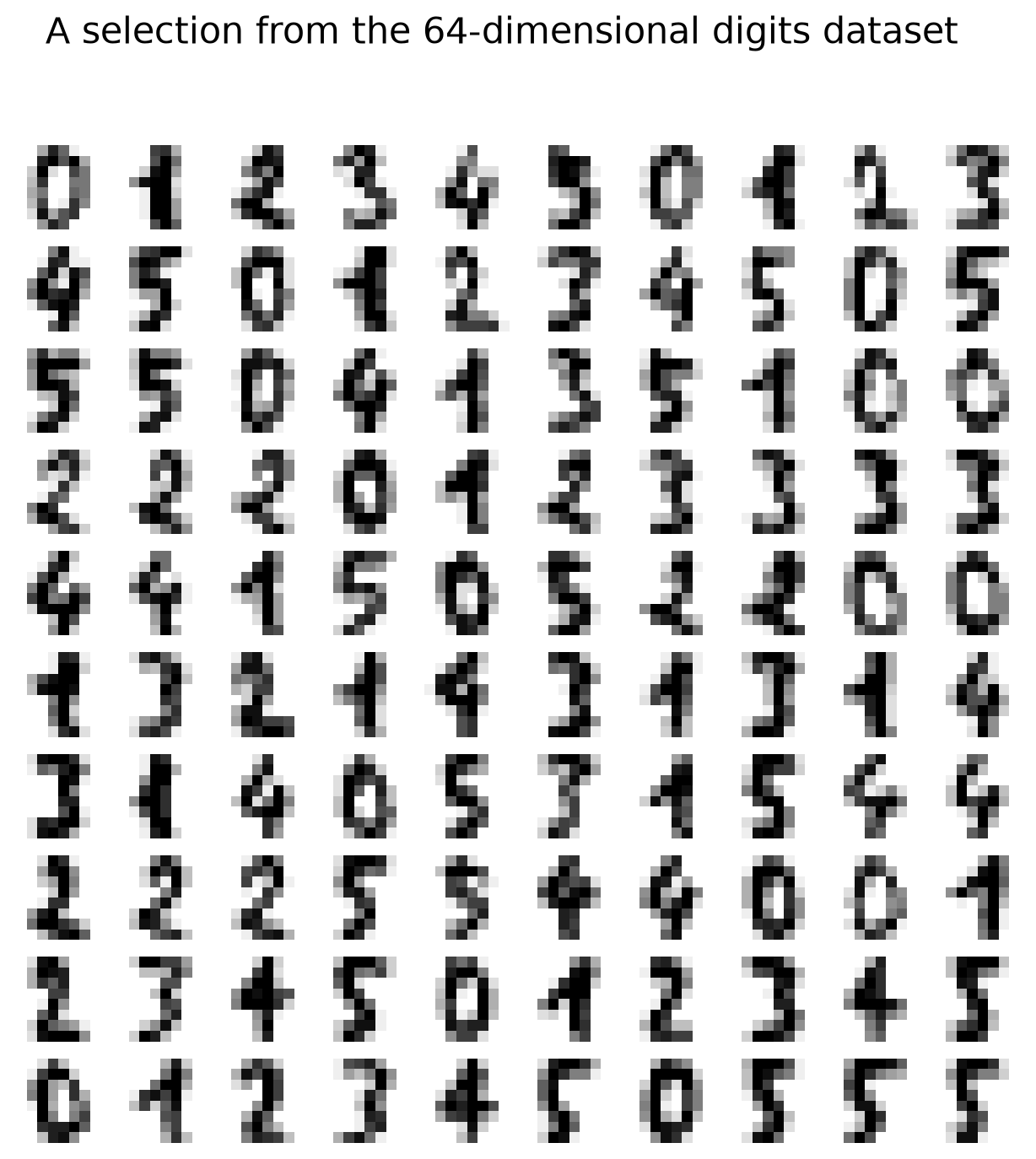
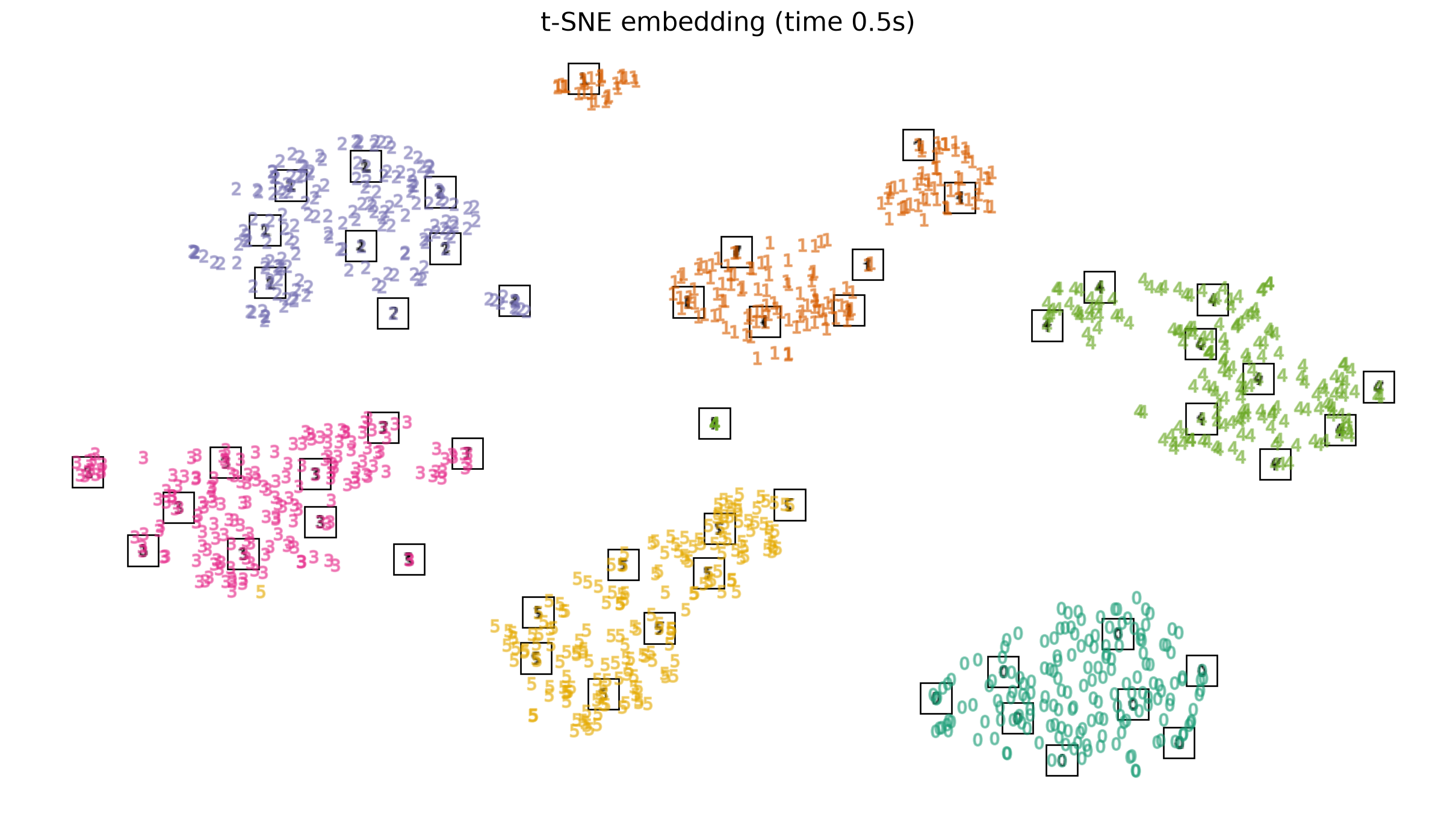
Digits: t-SNE embedding
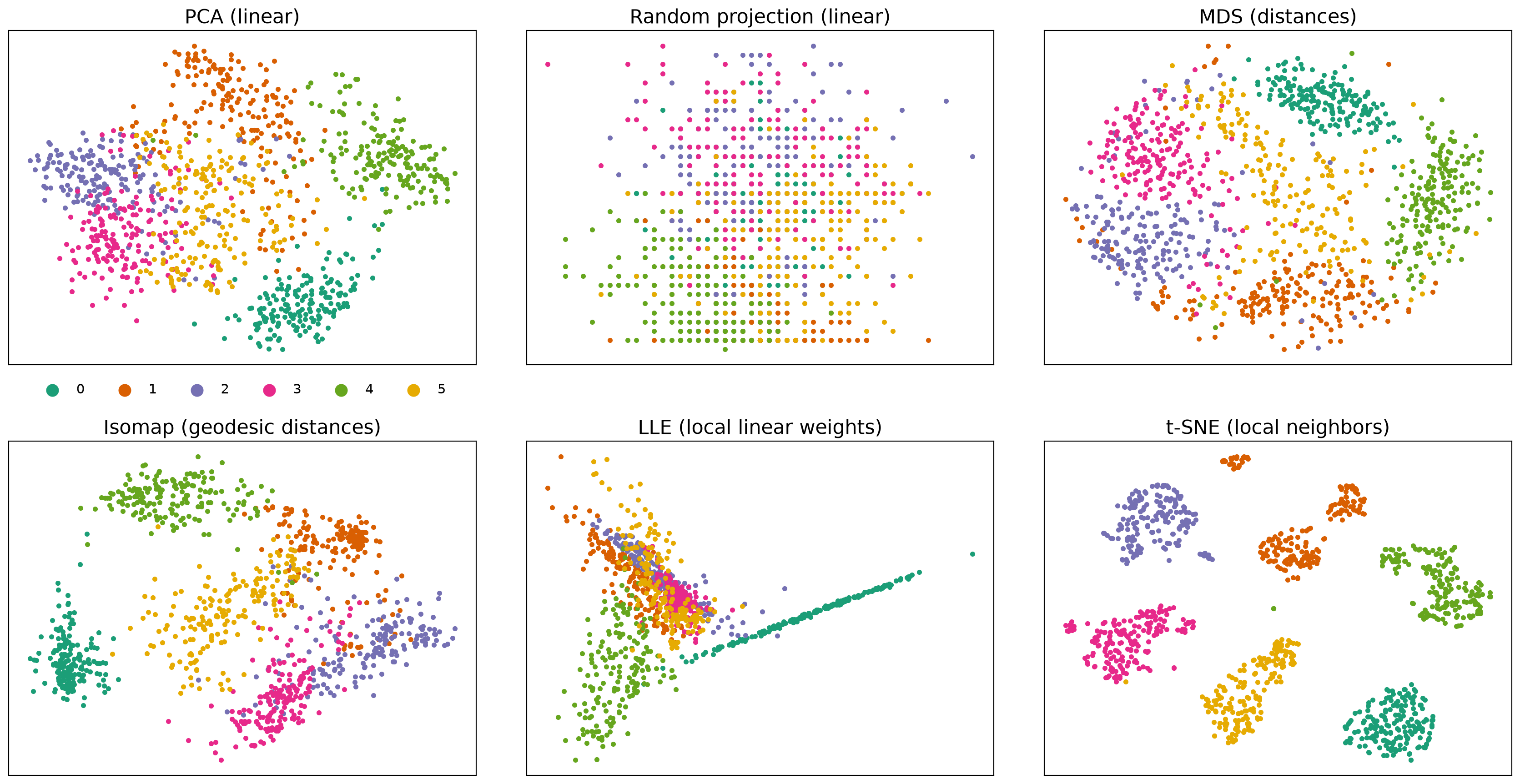
Same digits, six projections
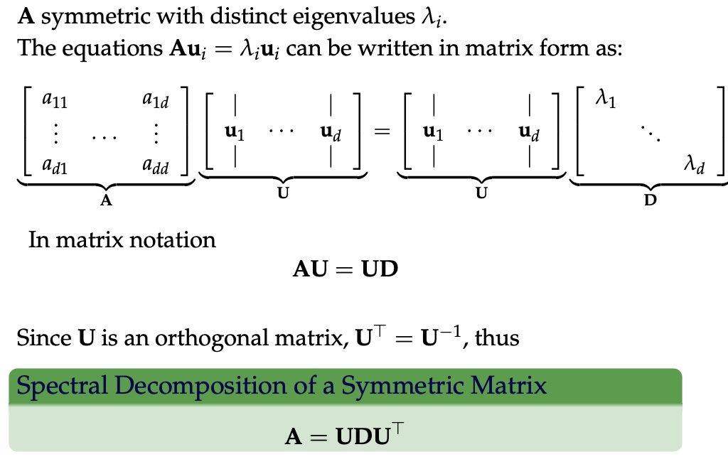
Symmetric Matrices
- \(\lambda \in \mathbb{R}\) and \(u \in \mathbb{R}^d\) (no complex numbers involved)
- The eigenvectors are orthogonal
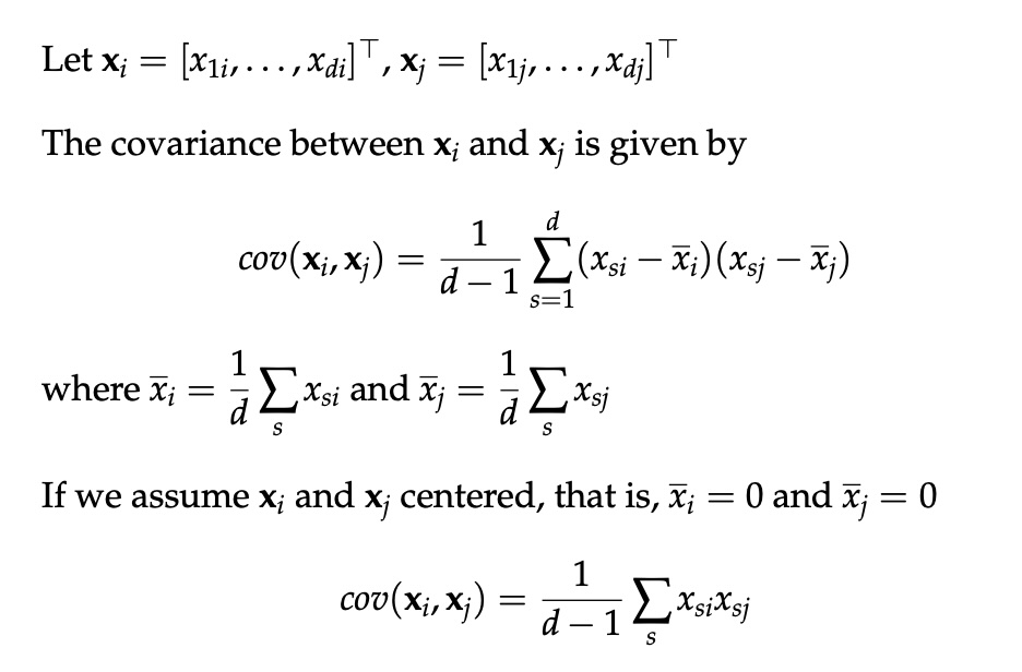
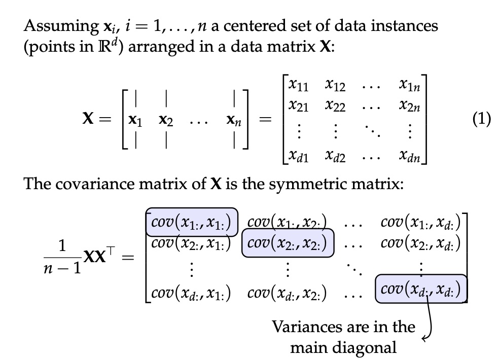
Covariance Matrix
Covariance Matrix
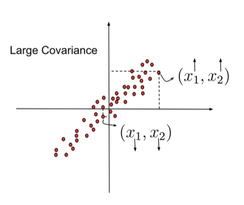
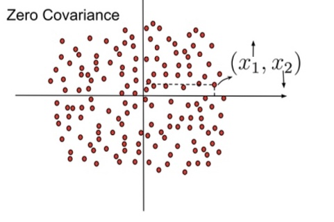
Covariance Matrix
Principal Component Analysis: intuition
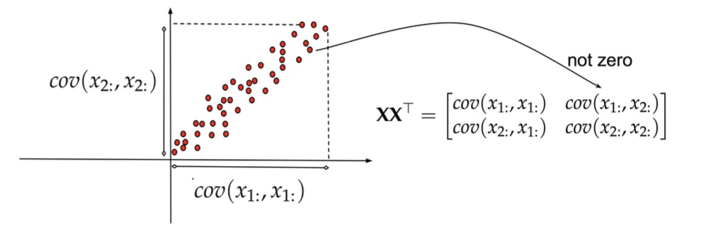
Principal Component Analysis: intuition
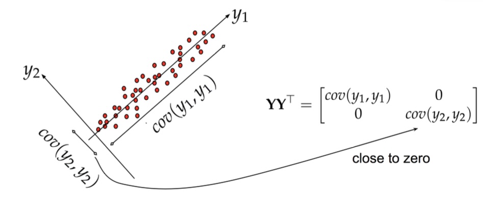
Principal Component Analysis
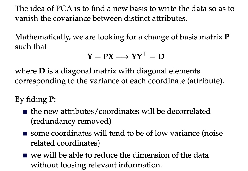
Principal Component Analysis
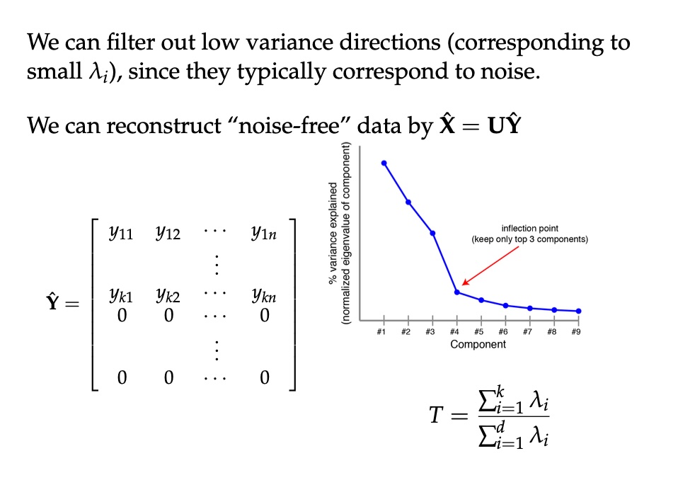
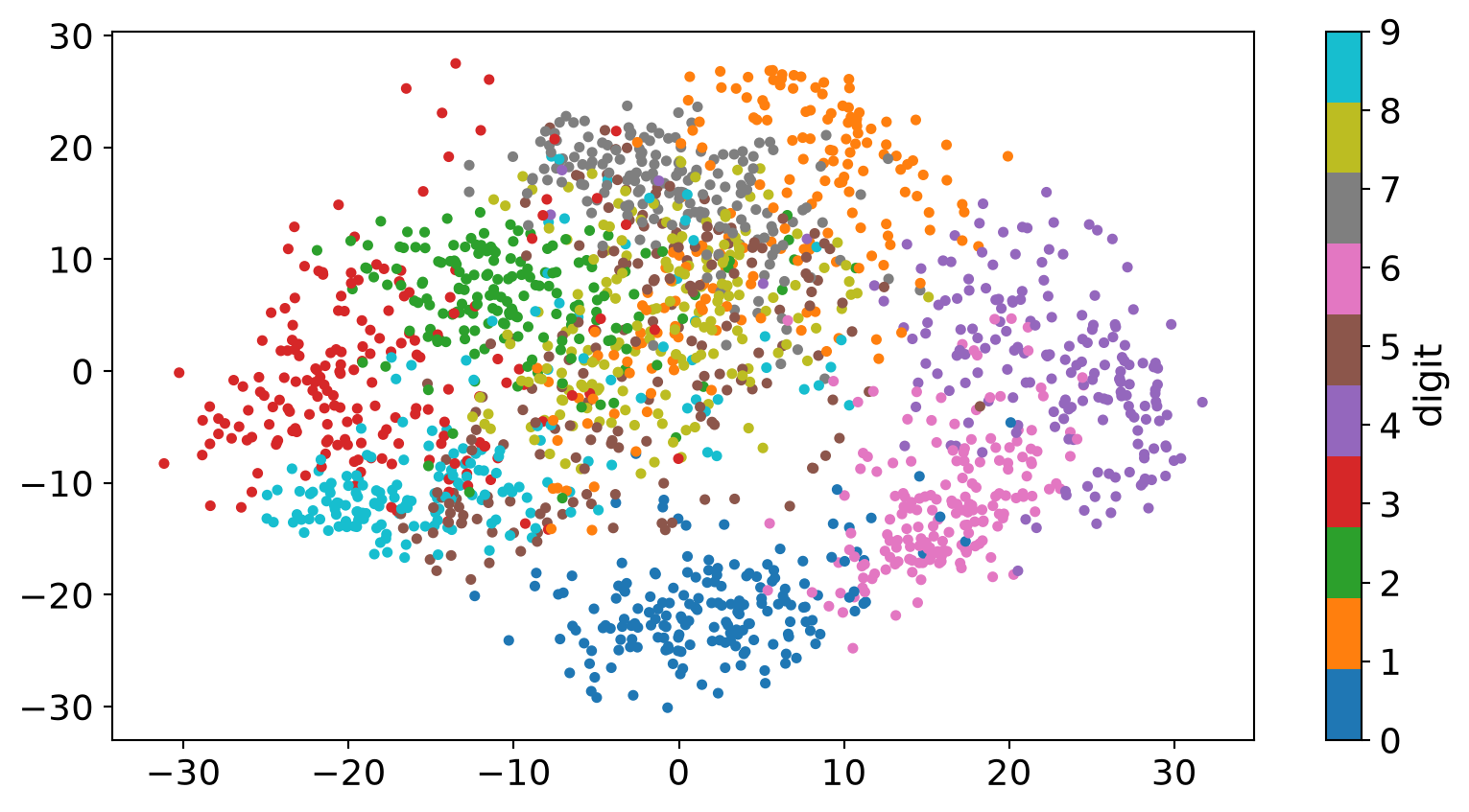
PCA of digits
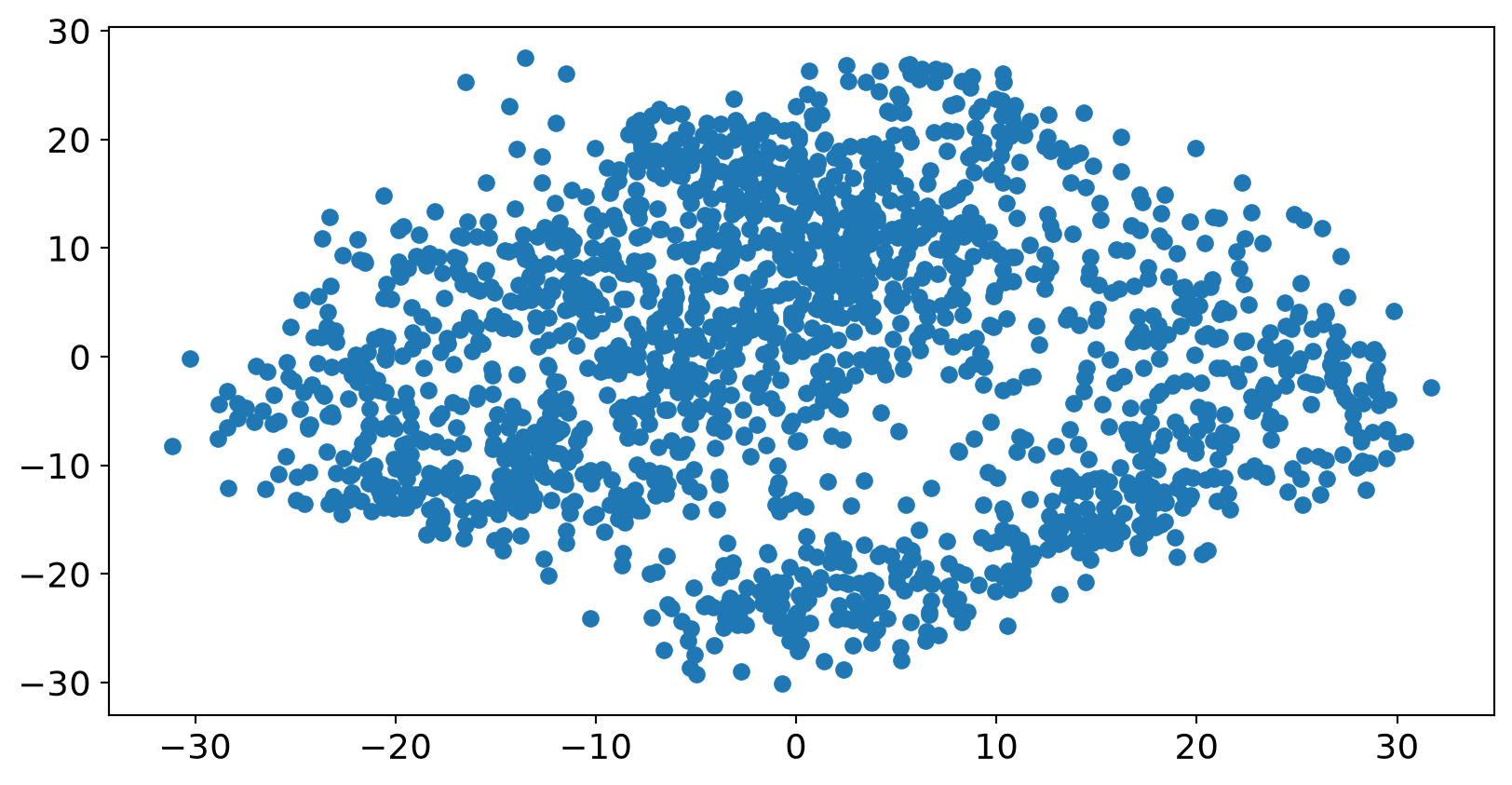
PCA of digits
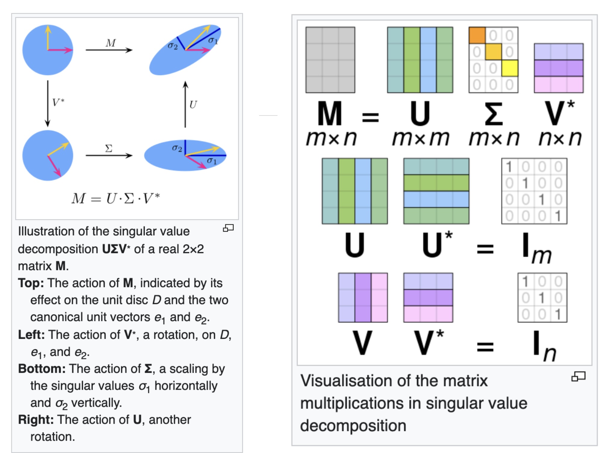
Singular Value Decomposition (SVD)
Any matrix, \(M = U \Sigma V^{*}\) — rotate, scale, rotate (Wikipedia)
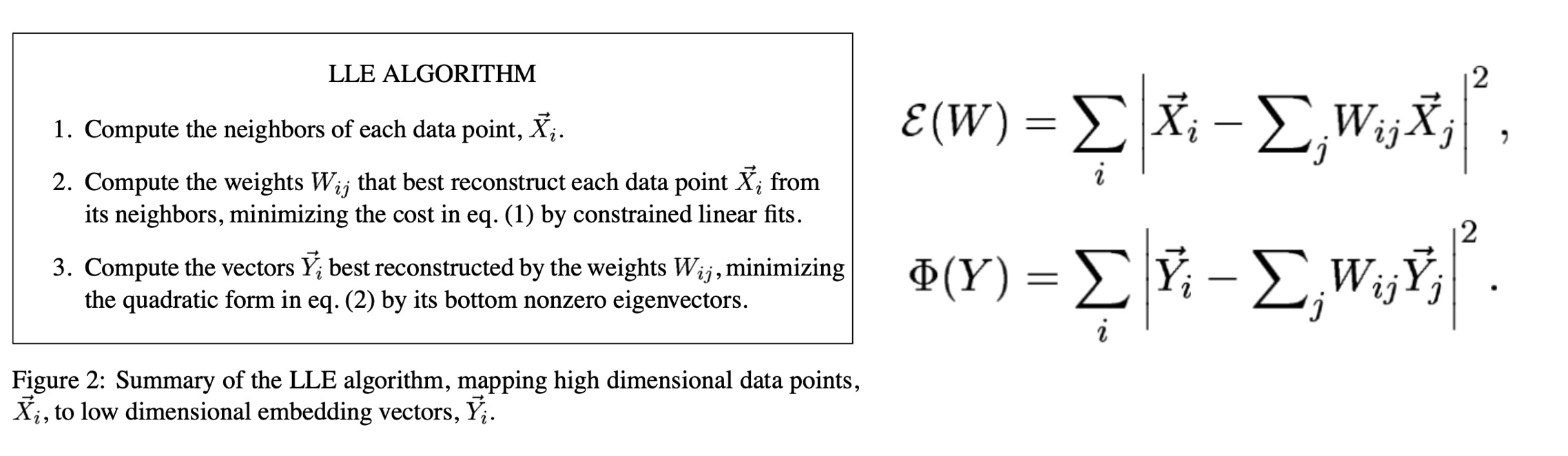
Local Linear Embedding
Preserving Local Manifold Neighborhoods
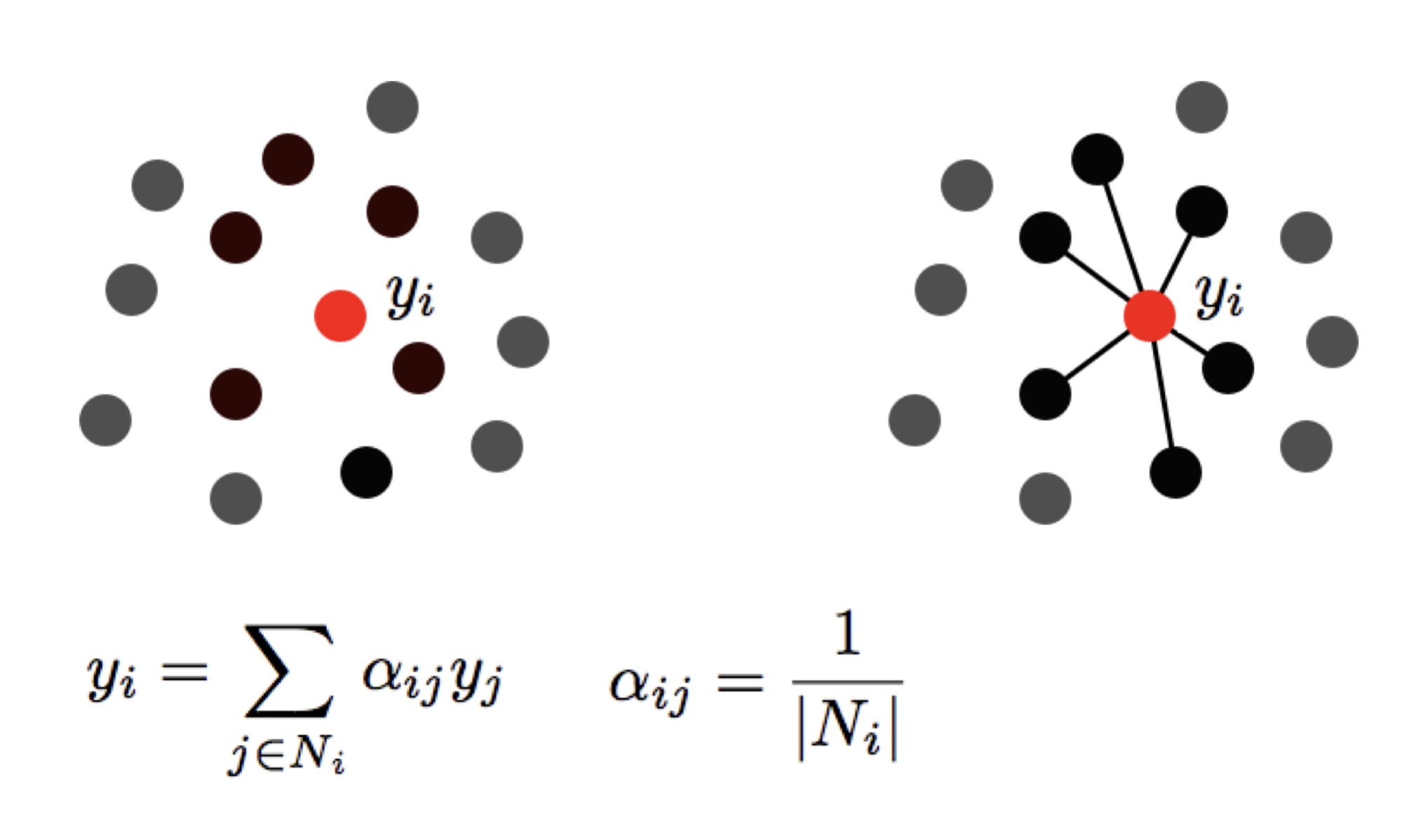
LLE
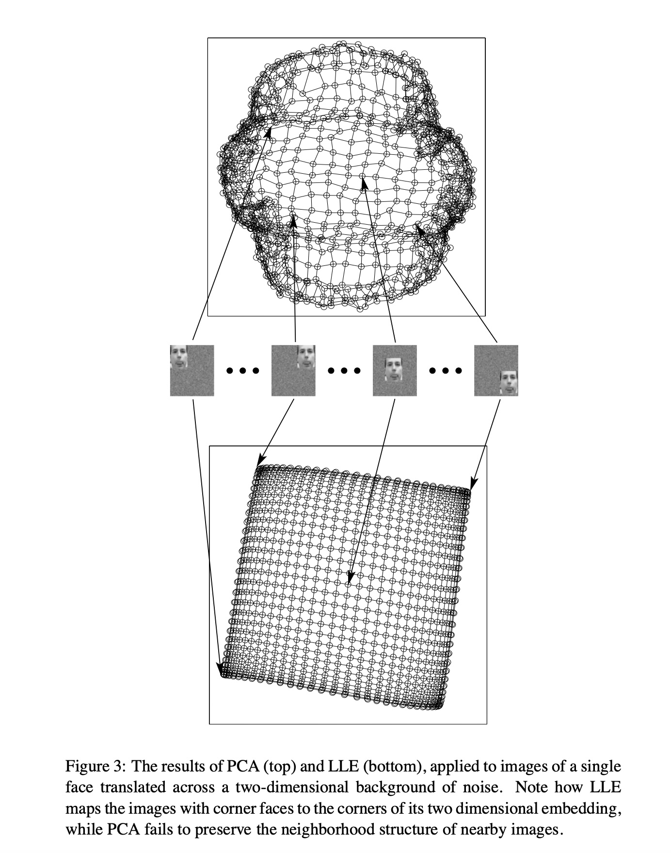
PCA vs LLE
- Images of one face translated across a noisy background: intrinsically 2-D (x and y position)
- PCA (top): folds the sheet; nearby images are not neighbors
- LLE (bottom): recovers a flat grid; corner faces map to corners