DS-GA 3001 - Fall 2026
NYU Center for Data Science
2026-10-27
Deep Learning Terminology and Foundations
Linear Models and Loss Functions
Shallow Neural Networks and Activation Functions
Deep Neural Networks and Composition
Interactive Visualization Tools
Acknowledgments:
Materials adapted from:
Understanding Deep Learning by Simon J.D. Prince
Published by MIT Press, 2023
Available free online: https://udlbook.github.io/udlbook
Why this book?

Prince, S. J. D. (2023). Understanding Deep Learning. MIT Press.
The Supervised Learning Framework:
\[y = f[x, \Phi]\]
| Symbol | Meaning | Example |
|---|---|---|
| \(y\) | Prediction (model output) | House price: $450,000 |
| \(x\) | Input (features) | Square footage: 2000 sq ft, Bedrooms: 3 |
| \(\Phi\) | Model parameters (weights, biases) | Millions of numbers learned from data |
| \(f[\cdot]\) | Model function (architecture) | Neural network with multiple layers |
Key Insight: Deep learning learns the parameters \(\Phi\) from training data pairs \(\{x_i, y_i\}\) to minimize prediction errors.
Training Data:
Pairs of inputs and outputs: \(\{x_i, y_i\}\)
Loss Function:
Quantifies prediction accuracy: \(L[\Phi]\)
Goal:
Find parameters \(\Phi\) that minimize \(L[\Phi]\)
\[\Phi^* = \arg\min_{\Phi} L[\Phi]\]
Generalization:
Test on separate data not seen during training
The Challenge:
We don’t want to just memorize training data!
We want models that generalize to new, unseen examples.
→ This is why we split data into train/validation/test sets.
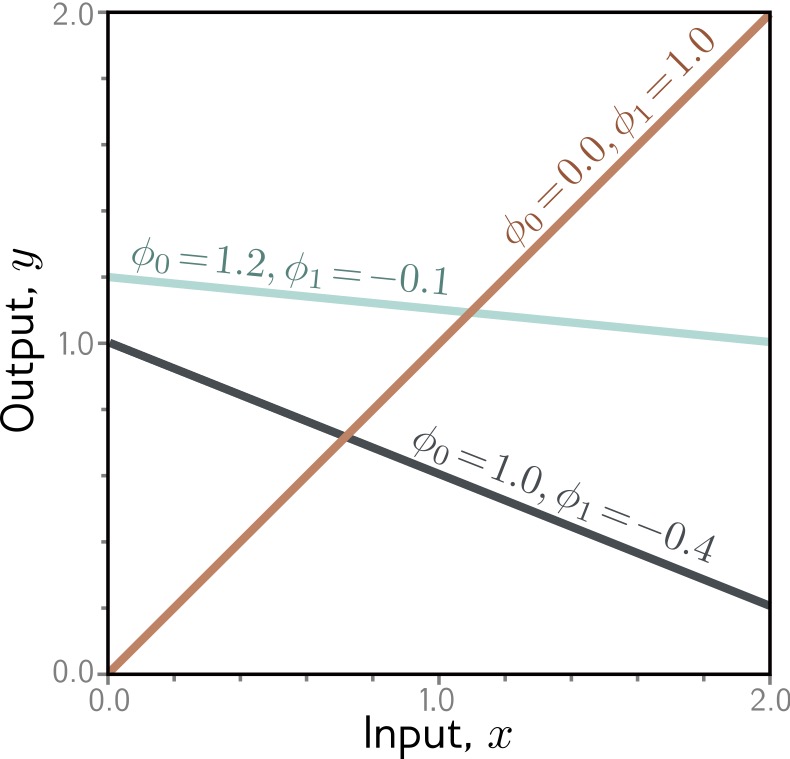
The simplest supervised learning model:
\[y = f[x, \Phi] = \Phi_0 + \Phi_1 x\]

Prince, S. J. D. (2023). Understanding Deep Learning. Chapter 2: Supervised Learning.
How do we quantify “good fit”?
Loss Function: Sum of squared errors
\[L[\Phi] = \sum_{i=1}^{N} (y_i - f[x_i, \Phi])^2\]
Vertical distance from each data point to the line → squared → summed = total error
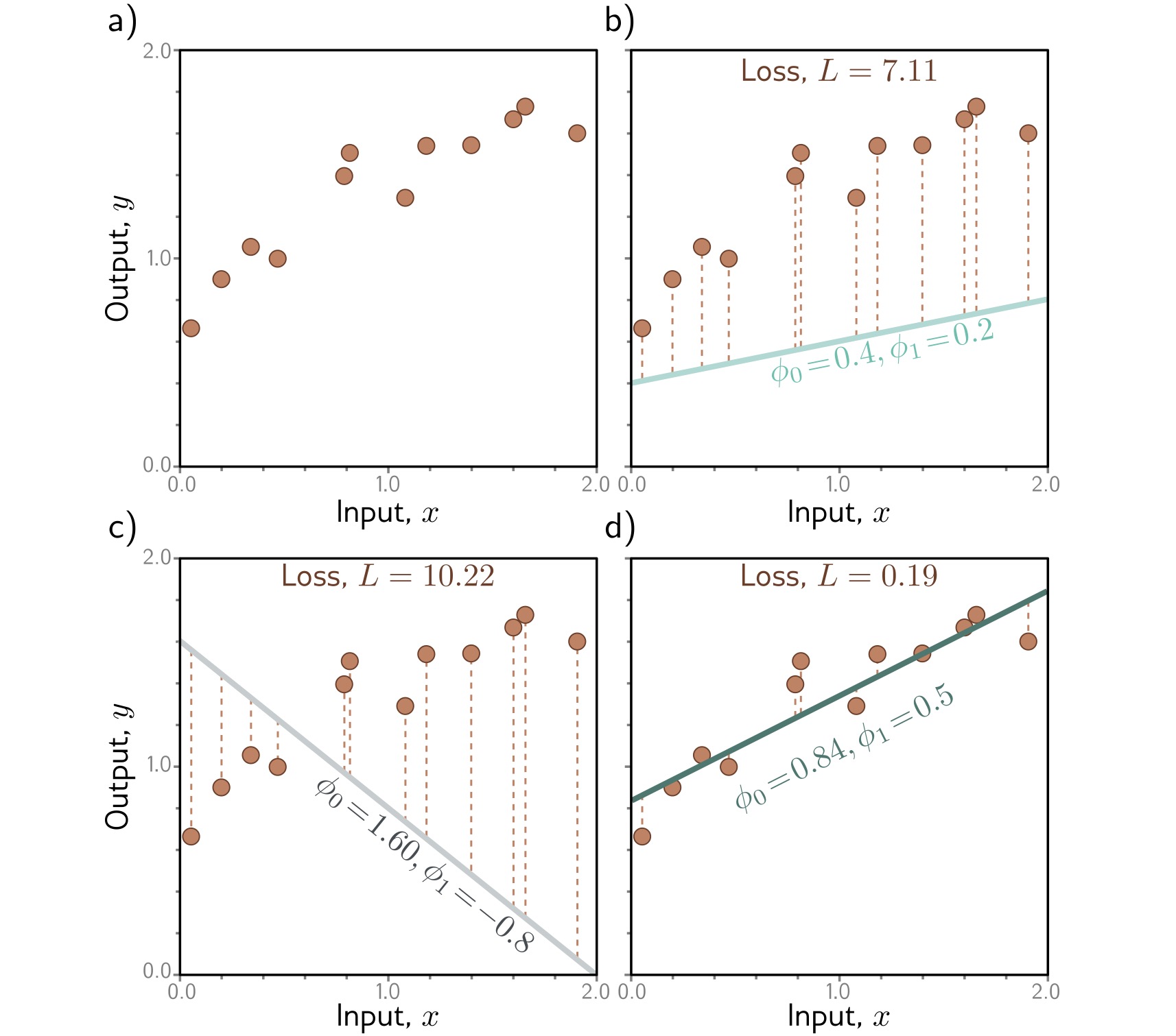
Prince, S. J. D. (2023). Understanding Deep Learning. Chapter 2: Supervised Learning.
Every point on the surface is one choice of parameters; we want the lowest point.
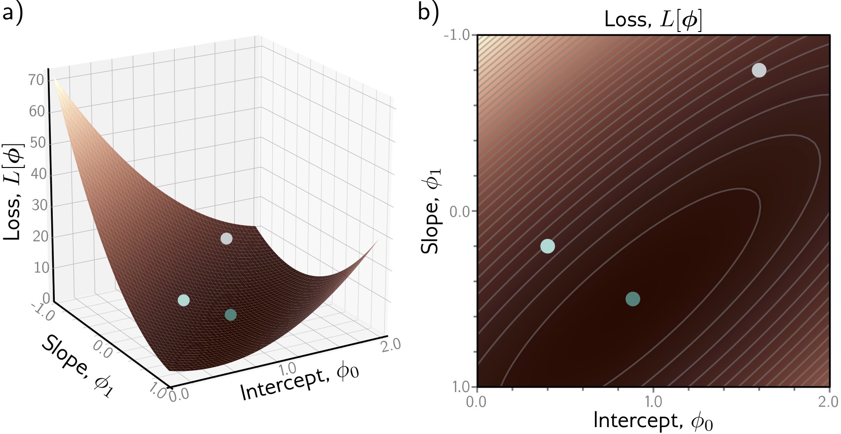
Prince, S. J. D. (2023). Understanding Deep Learning. Chapter 2: Supervised Learning.
Goal: Find the lowest point (the darkest region in panel b)
Key Observations:
For linear models, optimization is easy! Deep networks have much more complex loss landscapes…
Iteratively move downhill, opposite to the gradient.
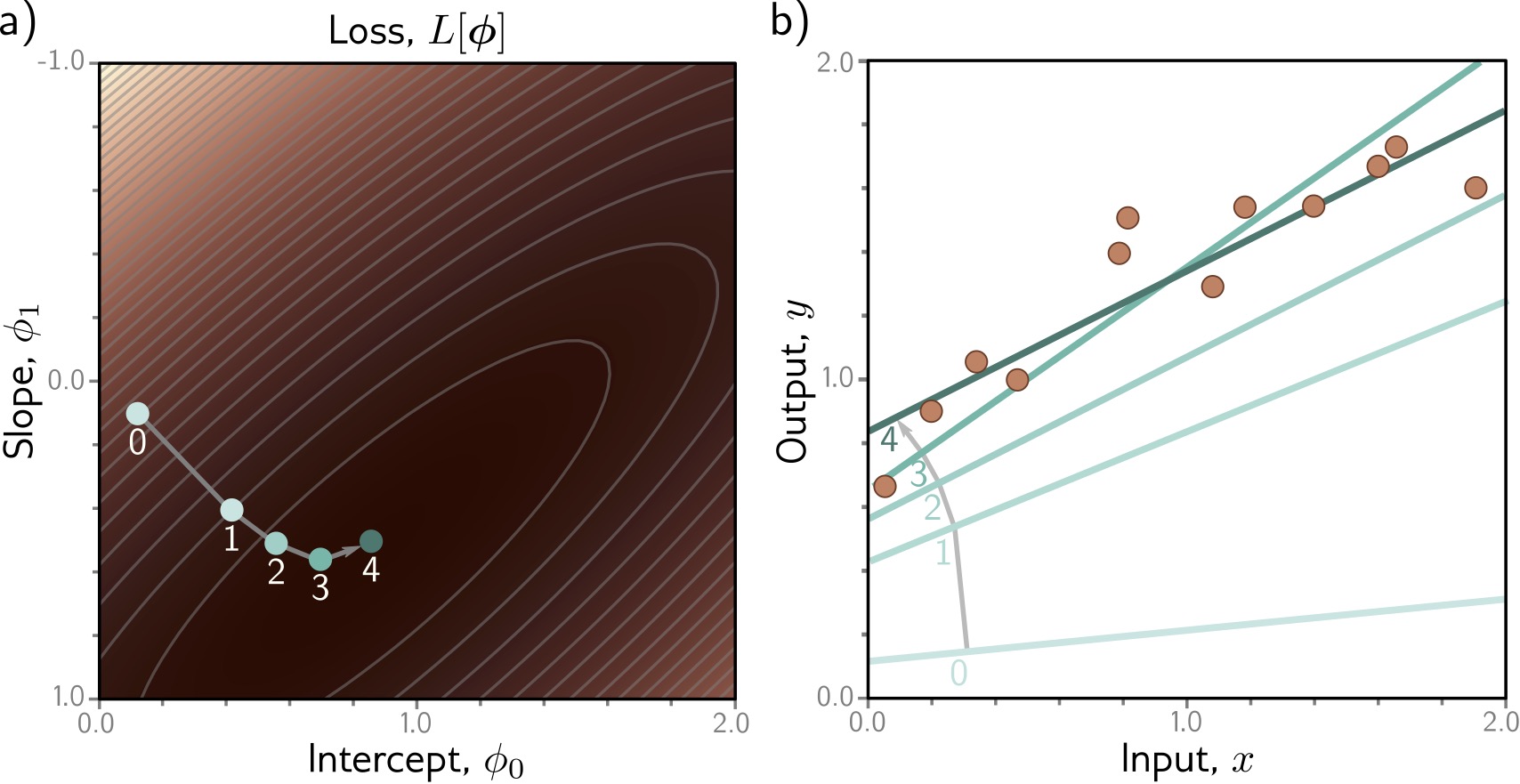
Prince, S. J. D. (2023). Understanding Deep Learning. Chapter 2: Supervised Learning.
How do we find the minimum?
\[\Phi_{new} = \Phi_{old} - \alpha \nabla L[\Phi]\]
\(\alpha\) = learning rate
Linear models are limited - they can only learn straight lines!
Solution: Add non-linearity through activation functions
Transform linear combinations with a non-linear function → enables learning complex patterns
Shallow Neural Network (1 hidden layer):
\[y = f[x, \Phi] = \Phi_0 + \sum_{i=1}^{3} \Phi_i \cdot a[ \Theta_{i0} + \Theta_{i1} x]\]
| Component | Description | Count |
|---|---|---|
| \(\Theta_{ij}\) | First layer parameters | 6 parameters |
| \(\Phi_i\) | Second layer parameters | 4 parameters |
| \(a[\cdot]\) | Activation function | Non-linearity! |
Total: 10 parameters (vs 2 for linear model)
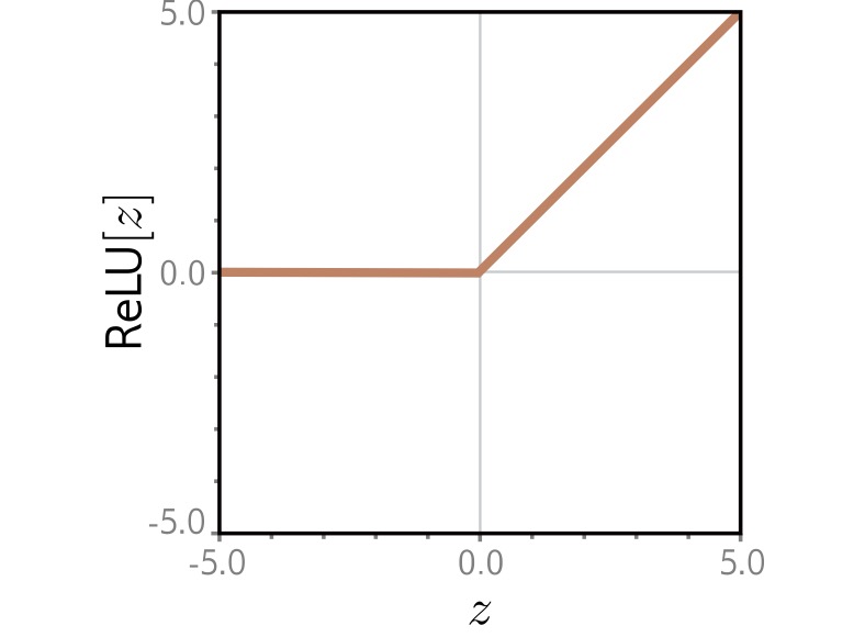
ReLU (Rectified Linear Unit): the most popular activation function
\[a[z] = \max(0, z) = \begin{cases} z & \text{if } z > 0 \\ 0 & \text{if } z \leq 0 \end{cases}\]
Why ReLU?

Prince, S. J. D. (2023). Understanding Deep Learning. Chapter 3: Shallow Neural Networks.
The same 3-hidden-unit network, with different parameters, produces three different piecewise-linear functions.
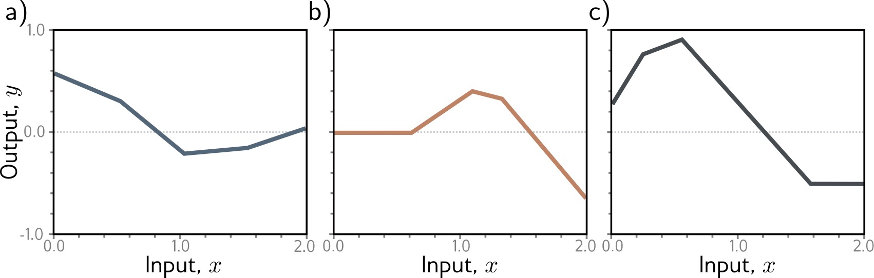
Prince, S. J. D. (2023). Understanding Deep Learning. Chapter 3: Shallow Neural Networks.
Each hidden unit:
Combining multiple units:
Step-by-step: how a shallow network processes an input
Input \(x\) (left) enters the network
Each hidden unit computes: \(h_i = a[\Theta_{i0} + \Theta_{i1} x]\)
Weighted combination: \(y = \Phi_0 + \sum_i \Phi_i h_i\)
Final output \(y\) (right)
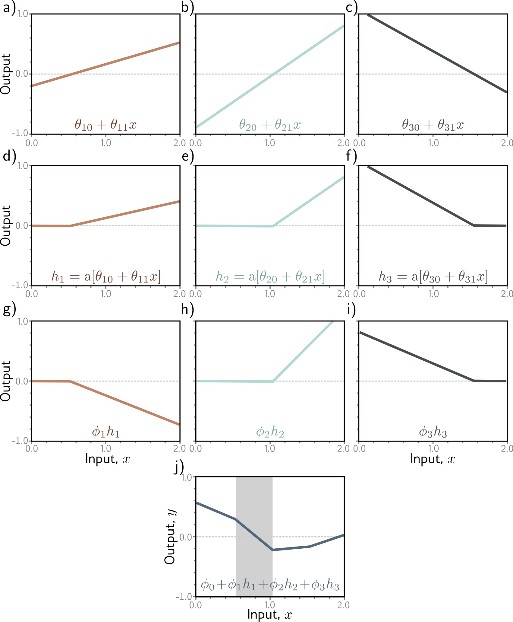
Prince, S. J. D. (2023). Understanding Deep Learning. Chapter 3: Shallow Neural Networks.
The standard picture: inputs feed hidden units, which feed the output.
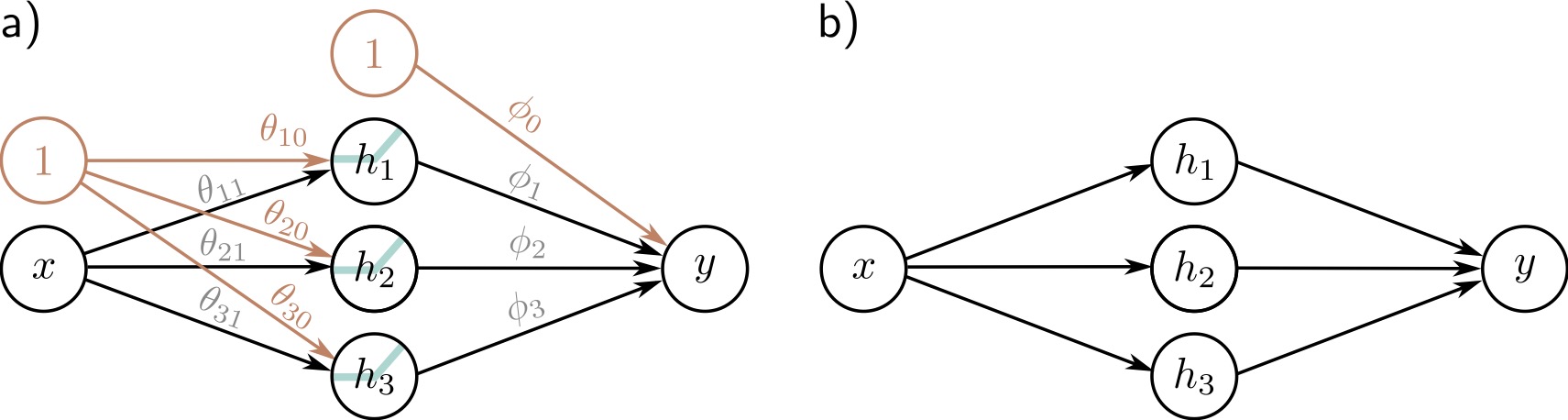
Prince, S. J. D. (2023). Understanding Deep Learning. Chapter 3: Shallow Neural Networks.
Components:
Terminology:
A shallow network with enough hidden units can approximate any continuous function.
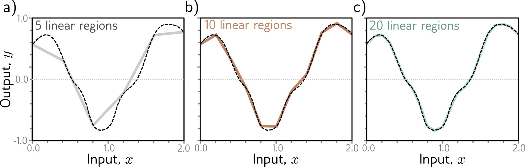
Cybenko, G. (1989). Approximation by superpositions of a sigmoidal function. Mathematics of Control, Signals and Systems, 2(4), 303-314.
Theorem (Cybenko 1989, Hornik 1991):
A shallow neural network with enough hidden units can approximate any continuous function to arbitrary accuracy on a compact domain.
But…
Cybenko, G. (1989). Approximation by superpositions of a sigmoidal function. Mathematics of Control, Signals and Systems, 2(4), 303-314.
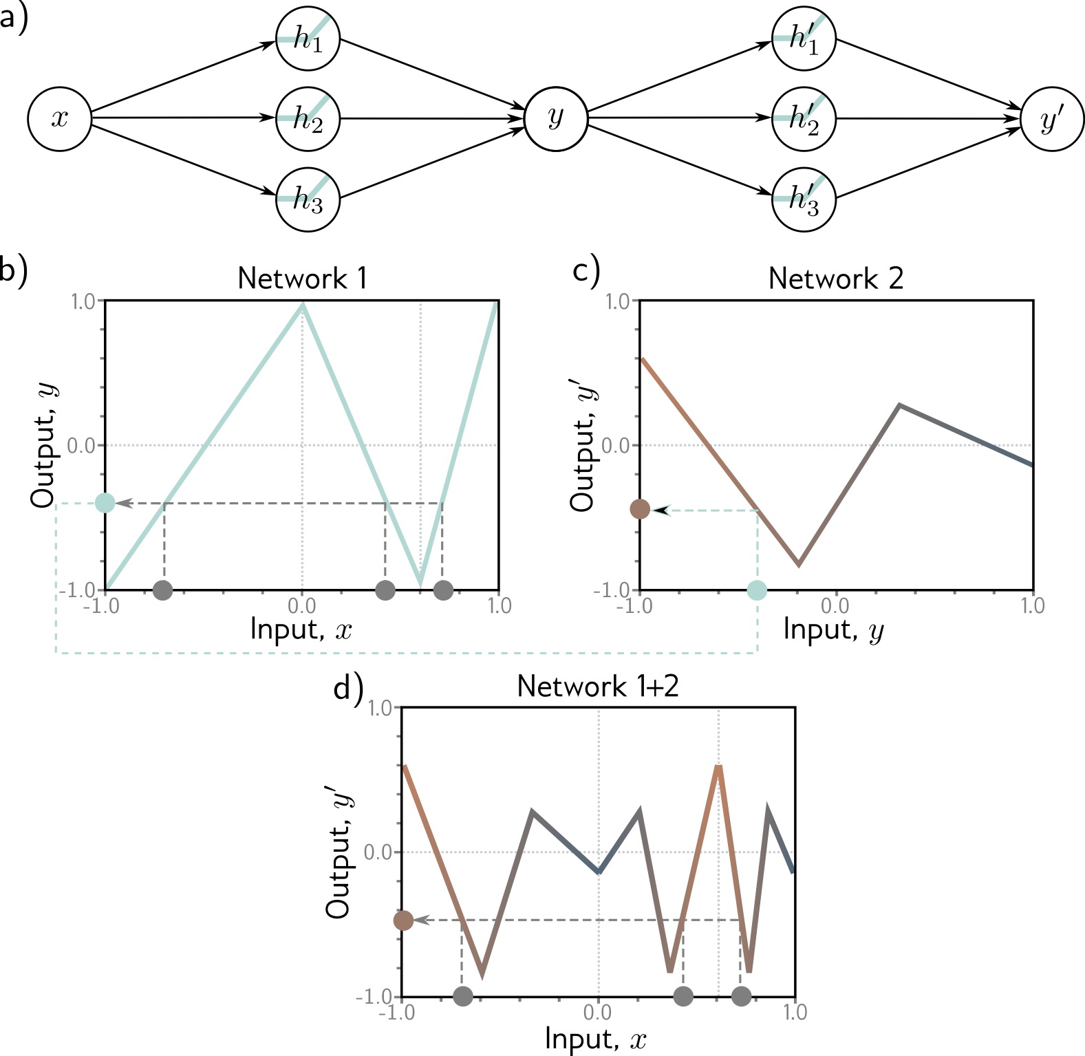
Deep networks compose simple transformations to build complex representations
Shallow network limitations:
Deep network advantages:
Intuition from vision:
Layer 1: Edges, colors
↓
Layer 2: Textures, simple shapes
↓
Layer 3: Object parts
↓
Layer 4: Object categories
Each layer builds on previous representations!
Building deep networks: stack multiple hidden layers
Each layer:
\[h^{(k)} = a[W^{(k)} h^{(k-1)} + b^{(k)}]\]

Prince, S. J. D. (2023). Understanding Deep Learning. Chapter 4: Deep Neural Networks.
Each layer bends and folds the representation space, pulling intertwined classes apart.
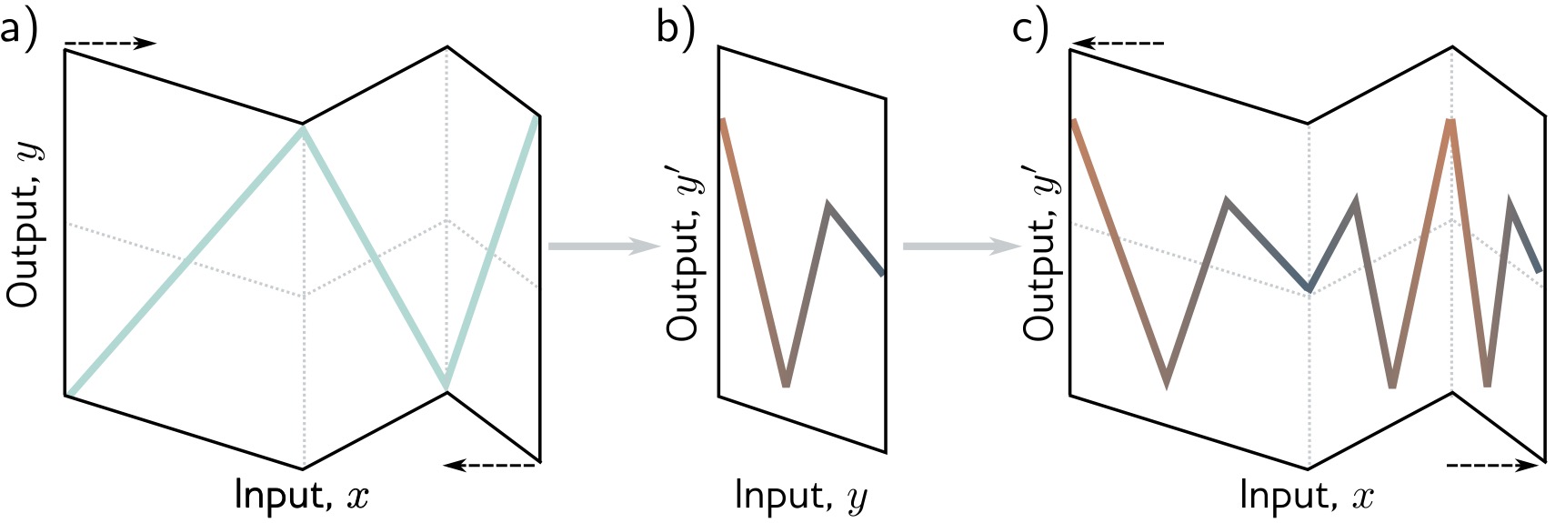
Prince, S. J. D. (2023). Understanding Deep Learning. Chapter 4: Deep Neural Networks.
Layer 1:
Stretches, rotates, bends space with ReLU
Layer 2:
Further transforms the already-bent space
Result:
Complex folding of input space
→ Can separate classes that were originally intertwined
The second layer operates on intermediate representations, not on raw inputs.
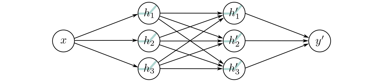
Prince, S. J. D. (2023). Understanding Deep Learning. Chapter 4: Deep Neural Networks.
Example: First layer detects edges, second layer combines edges into shapes
Modern deep learning: many layers stacked, each building on the last.
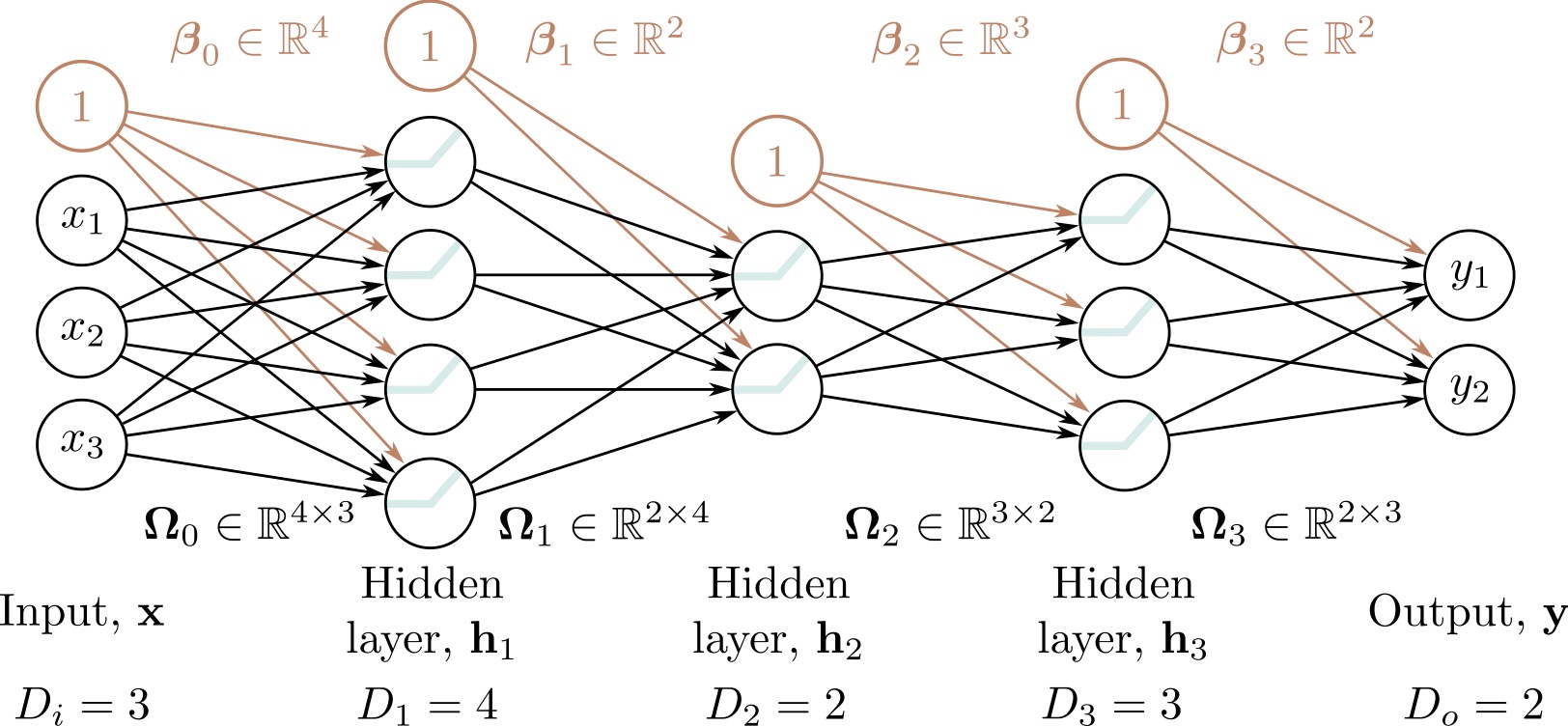
Prince, S. J. D. (2023). Understanding Deep Learning. Chapter 4: Deep Neural Networks.
Modern architectures: ResNet (152 layers), GPT-3 (96 layers), Vision Transformers (24+ layers)
Interactive tool for understanding neural networks · https://playground.tensorflow.org
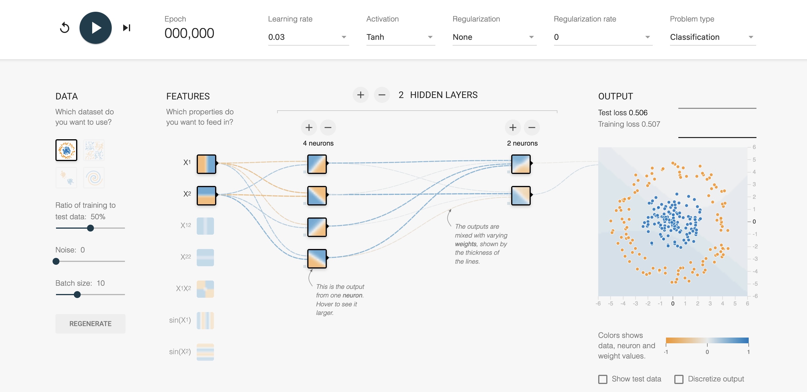
Smilkov, D., & Carter, S. (2016). TensorFlow Playground. Google Brain.
Interactive visualization of Convolutional Neural Networks · https://poloclub.github.io/cnn-explainer/
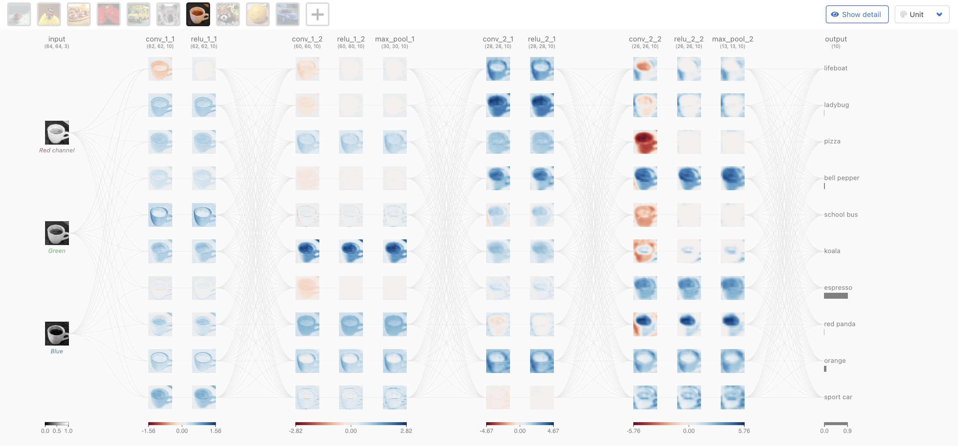
Wang, Z. J., et al. (2020). CNN Explainer: Learning Convolutional Neural Networks with Interactive Visualization. IEEE VIS.
Recommended interactive visualizations and resources:
Neural Network Visualization:
Distill.pub: The Building Blocks of Interpretability Comprehensive visual explanations
TensorFlow Embedding Projector Explore high-dimensional embeddings
ML4A: Looking Inside Neural Nets Interactive tutorials and visualizations
Understanding Deep Learning:
Free online textbook with: - Interactive Python notebooks - Video lectures - Extensive visualizations - Modern coverage (transformers, diffusion models)
Key Takeaways:
Supervised Learning: Learn parameters \(\Phi\) from data pairs \(\{x_i, y_i\}\) to minimize loss \(L[\Phi]\)
From Linear to Non-linear: Activation functions (ReLU) enable learning complex patterns
Shallow Networks: Single hidden layer can approximate any function (Universal Approximation Theorem)
Deep Networks: Multiple layers learn hierarchical representations more efficiently
Geometric View: Networks transform input space through non-linear folding to separate classes
Next lectures: We’ll explore specialized visualizations for CNNs, attention mechanisms, activation analysis, and network interpretability
Preview of upcoming topic:
Language models are deep networks too
Why it matters:
Today’s building blocks (layers, activations, learned representations) are what transformers are made of.
Next week we ask how to see what a language model is doing.