## Today ```{python} #| include: false import warnings warnings.filterwarnings("ignore") import numpy as np import matplotlib.pyplot as plt from sklearn.decomposition import MiniBatchDictionaryLearning plt.rcParams.update({"font.size": 20, "axes.spines.top": False, "axes.spines.right": False, "axes.titlesize": 22, "legend.frameon": False}) PURPLE, VIOLET, GRAY, ORANGE, TEAL, RED = "#57068c", "#8900e1", "#6d6d6d", "#e08214", "#1b9e77", "#c62828" FCOL = [PURPLE, ORANGE, TEAL, RED, "#1f78b4"] # one color per feature in the 5-feature model # The toy model of Elhage et al. (2022), "ReLU output" variant: # h = W x (n features squeezed into m < n hidden dimensions) # x' = ReLU(W^T h + b) # trained to reconstruct x under an importance-weighted squared error. Each feature x_i is 0 with # probability S (the sparsity) and uniform on [0, 1] otherwise. Plain numpy with Adam. def sample(rng, size, n, S): return rng.uniform(0, 1, (size, n)) * (rng.uniform(0, 1, (size, n)) > S) def train(n, m, S, imp, steps=4000, batch=1024, lr=1e-2, seed=0): rng = np.random.default_rng(seed) W = rng.normal(0, 0.3, (m, n)); b = np.zeros(n) mW = np.zeros_like(W); vW = np.zeros_like(W); mb = np.zeros(n); vb = np.zeros(n) for t in range(1, steps + 1): X = sample(rng, batch, n, S) H = X @ W.T; Z = H @ W + b; Y = np.maximum(Z, 0) G = -2 * imp * (X - Y) * (Z > 0) / batch gW = H.T @ G + (G @ W.T).T @ X; gb = G.sum(0) for p, g, mm, vv in ((W, gW, mW, vW), (b, gb, mb, vb)): mm *= 0.9; mm += 0.1 * g; vv *= 0.999; vv += 0.001 * g * g p -= lr * (mm / (1 - 0.9 ** t)) / (np.sqrt(vv / (1 - 0.999 ** t)) + 1e-8) X = sample(rng, 20000, n, S) loss = float((imp * (X - np.maximum(X @ W.T @ W + b, 0)) ** 2).sum(1).mean()) return W, b, loss def best_of(n, m, S, imp, seeds=4, **kw): return min((train(n, m, S, imp, seed=s, **kw) for s in range(seeds)), key=lambda r: r[2]) # Five features in two dimensions, at three sparsity levels (used on several slides). IMP5 = 0.9 ** np.arange(5) TOY5 = {S: best_of(5, 2, S, IMP5) for S in (0.0, 0.8, 0.9)} N_REP = {S: int((np.linalg.norm(TOY5[S][0], axis=0) > 0.5).sum()) for S in TOY5} ``` 1. **Why look inside?** From explaining an output to understanding a mechanism 2. **Superposition**: why single neurons are hard to read 3. **From neurons to features**: dictionary learning and the replacement model 4. **Attribution graphs**: drawing one prompt's computation as a graph 5. **Case studies**: reasoning, planning, hallucination, chain of thought 6. **Attention**: the part those graphs leave out, and filter heads 7. **Limits**: what these pictures can and cannot claim *This is the last regular lecture. It replaces the session on fairness.* ::: {.notes} TIMING (120 min): part 1 about 10 min, part 2 about 25, part 3 about 15, part 4 about 20, part 5 about 25, part 6 about 15, part 7 about 10. Four sources carry the lecture. Toy Models of Superposition (Elhage et al., 2022) for part 2. Circuit Tracing (Ameisen et al., 2025) for parts 3 and 4. On the Biology of a Large Language Model (Lindsey et al., 2025) for part 5. LLMs Process Lists With General Filter Heads (Sen Sharma et al., 2025) for part 6. The first three are from Anthropic's interpretability team; the fourth is from David Bau's lab at Northeastern. The charts in part 2 are computed in this deck from a model small enough to train in seconds. Everything in parts 4 to 6 is a figure from the papers. ::: # Why Look Inside? ## Where we left off on November 3 :::: {.columns} ::: {.column width="50%"} **What we had** * **Embeddings**: words as points, neighbors as meaning * **Attention maps**: which tokens a head looks at * **LIME**: which input words move the output **What the lab found** * A classifier can be right for the wrong reason * An attention map shows where a head looks. It does not show what was computed with what it found. ::: ::: {.column width="50%"} **Three levels of explanation** 1. **Behavior**: what does the model output? (evaluation) 2. **Attribution**: which inputs mattered for this output? (LIME, SHAP, saliency) 3. **Mechanism**: what intermediate steps did the model compute? (today) **Level 3 is what would let us say *how* an answer was produced, and check whether the model's own explanation is true.** ::: :::: ::: {.notes} Three weeks ago we looked at an NLP model from the outside in: its embeddings, its attention, and input attributions with LIME. The lab ended on a question, 'does attention explain the prediction?', and the honest answer was 'only partly'. Attention tells you which positions information was read from. It says nothing about what the information was or what happened to it next. Today is about the third level. The goal is ambitious: take one prompt and one answer, and draw the intermediate steps the model actually went through. The field is called mechanistic interpretability. It is also a visualization lecture. Every method today ends in a picture, and the papers say outright that the interface was one of the main contributions. ::: ## A transformer in one slide :::: {.columns} ::: {.column width="55%"} * Every token position carries a vector, the **residual stream**. Each layer reads it and adds to it. * **Attention** moves information between positions. * **MLP layers** compute new information at one position. Their hidden units are the **neurons**. * At the last position, the final vector is turned into scores (**logits**) for the next token. **So there are two things to explain: what is represented in those vectors, and how each layer transforms it.** ::: ::: {.column width="45%"} ``` logits -> next token ^ [ layer L ] attention + MLP ^ ... ^ [ layer 2 ] attention + MLP ^ [ layer 1 ] attention + MLP ^ token embeddings ``` ::: :::: ::: {.notes} A reminder of the architecture, at the level of detail today needs. You saw the full version in the Transformer Explainer lab. The picture to keep is a column of vectors per token, with each layer adding its contribution. Attention is the only component that moves information sideways, from one token to another. The MLP works on each position alone. Most of today's work is about the MLPs: that is where the neurons are, and they hold most of the parameters. Attention comes back in part 6 as the thing the main method cannot explain. ::: # Superposition ## The hope: one neuron, one concept :::: {.columns} ::: {.column width="50%"} **If it held** * Read a neuron's top-activating examples, name it, done * Some neurons really are like this: curve detectors in vision models, for example **What people found in language models** * Most neurons are **polysemantic**: one neuron responds to several unrelated things * Top activations can look clean while weaker activations mean something else ::: ::: {.column width="50%"} **Two questions from the paper** * Why do neurons sometimes line up with concepts and sometimes not? * Can a network represent **more features than it has neurons**? **The answer to the second is yes, and it explains the first.** ::: :::: :::footer Elhage, N., et al. (2022). [*Toy Models of Superposition*](https://transformer-circuits.pub/2022/toy_model/index.html). Transformer Circuits Thread. ::: ::: {.notes} The simplest plan for interpretability is to look at neurons one at a time. In early vision models this worked surprisingly often. In language models it mostly fails. A typical neuron fires on, say, academic citations, Korean text and HTTP requests. That is what 'polysemantic' means. There is no single label for it. Toy Models of Superposition asks why. Its move is to stop studying real networks, where nobody knows what the true features are, and build a tiny one where the features are known by construction. ::: ## Features are directions * **Feature**: a property of the input the network represents (a curve, the word being in French, a mention of Texas) * **Linear representation hypothesis**: each feature has a **direction** in activation space. Several active features add up: $$\text{activation} \;=\; x_1 W_1 + x_2 W_2 + \dots$$ * The classic evidence: `king - man + woman ≈ queen` in word embeddings * A **neuron** is one particular direction: a coordinate axis. Nothing forces features to lie along the axes. **With m dimensions there are only m orthogonal directions. But there are far more than m features worth representing.** ::: {.notes} Two definitions carry the rest of the lecture. A feature is something the model represents about its input. The paper is careful that a clean definition is hard, and settles for a working one. The hypothesis is that features are directions, and that a vector is a weighted sum of the directions of the features that are present. You have seen the evidence: the embedding arithmetic from the NLP lecture, and the custom-axis exercise in the Embedding Projector. Now the tension. A language model plausibly wants to represent every person, place and concept it has read about. That is many more features than it has dimensions. If features must be orthogonal, most of them cannot be stored. So what happens? ::: ## How many directions fit in d dimensions? ```{python} #| fig-align: center rng = np.random.default_rng(0) fig, axes = plt.subplots(1, 3, figsize=(17, 5.6), sharey=True) for ax, d in zip(axes, (3, 100, 1000)): V = rng.normal(size=(2000, d)); V /= np.linalg.norm(V, axis=1, keepdims=True) C = (V @ V.T)[np.triu_indices(2000, 1)] ax.hist(C, bins=np.linspace(-1, 1, 81), color=PURPLE, alpha=0.85, weights=np.ones_like(C) / len(C)) ax.set_title(f"d = {d}\n{100 * np.mean(np.abs(C) < 0.1):.0f}% of pairs within ±0.1") ax.set_xlabel("cosine similarity") ax.axvspan(-0.1, 0.1, color=ORANGE, alpha=0.15) axes[0].set_ylabel("share of pairs") plt.tight_layout(); plt.show() ``` **Exactly orthogonal directions: only d. Almost orthogonal directions: enormously many, once d is large.** ::: {.notes} Computed here: 2,000 random directions in 3, 100 and 1,000 dimensions, and the cosine similarity of every pair. The shaded band is 'nearly orthogonal', within 0.1 of zero. In 3 dimensions random directions point all over the place. In 100 dimensions most pairs are already close to orthogonal. In 1,000 dimensions essentially all of them are. This is the geometric fact that makes superposition possible. A model's residual stream has thousands of dimensions. It has room for a huge number of directions that almost do not interfere. The price is the word 'almost': every feature leaks a little into the others. ::: ## A toy model with known features :::: {.columns} ::: {.column width="52%"} **Data: n synthetic features** * Each feature $x_i$ is **0 with probability S** (the *sparsity*), otherwise uniform on [0, 1] * Each has an **importance** $I_i$: how much its error counts **Model: squeeze n features into m < n dimensions and get them back** $$h = Wx \qquad x' = \mathrm{ReLU}(W^{\top}h + b)$$ $$L = \sum_i I_i\,(x_i - x'_i)^2$$ ::: ::: {.column width="48%"} **How to read the result** * Column $W_i$ is the **direction** given to feature *i* * Its **length** says whether the feature is represented at all * The **angles** between columns say which features interfere **We know the true features, so we can see exactly what the network did with them.** ::: :::: :::footer Elhage, N., et al. (2022). [*Toy Models of Superposition*](https://transformer-circuits.pub/2022/toy_model/index.html). Transformer Circuits Thread. ::: ::: {.notes} The setup of the paper's first experiment. It is an autoencoder with a bottleneck, and one ReLU at the output. The inputs stand for the features of an imagined, much larger network in which every feature has its own neuron. The question is what a small network does when it has to carry those features through fewer dimensions. Two knobs. Sparsity S: how rarely each feature is active. Real features are sparse: most tokens are not about Texas. Importance: some features reduce the loss more than others. The same matrix W is used to encode and to decode, so column i of W is unambiguously 'the direction of feature i'. Without the ReLU this is a linear autoencoder and the answer is known: it keeps the top m features, like PCA, and drops the rest. The ReLU changes that. ::: ## Five features in two dimensions ```{python} #| fig-align: center fig, axes = plt.subplots(1, 3, figsize=(17, 6.2)) for ax, S in zip(axes, (0.0, 0.8, 0.9)): W = TOY5[S][0] for i in range(5): ax.plot([0, W[0, i]], [0, W[1, i]], lw=4, color=FCOL[i], solid_capstyle="round") ax.scatter(W[0, i], W[1, i], s=110, color=FCOL[i], zorder=3) ax.set_xlim(-1.35, 1.35); ax.set_ylim(-1.35, 1.35); ax.set_aspect("equal") ax.set_xticks([]); ax.set_yticks([]) for sp in ax.spines.values(): sp.set_visible(True); sp.set_color("#cccccc") active = "always active" if S == 0 else f"active {100 * (1 - S):.0f}% of the time" ax.set_title(f"features {active}\n{N_REP[S]} of 5 represented") plt.tight_layout(); plt.show() ``` **Dense features: the model keeps two, at right angles, and drops three. Sparse features: it keeps all five, as a pentagon.** ::: {.notes} Computed in this deck: the same model trained three times, changing only how often the features are active. Each line is the direction the model assigned to one feature; a feature with no line was given length zero. Left, features always on: two dimensions, two features, orthogonal. The three least important features are not represented. This is what PCA would do. Middle, each feature on 20 percent of the time: four features, in two opposite pairs. A pair shares one dimension, pointing in opposite directions. Right, 10 percent: all five, evenly spaced around a circle. This is superposition: more features than dimensions. Nobody told the model to do it. It falls out of gradient descent once the features are sparse enough. The paper reports the same pentagon. ::: ## What the hidden activations look like ```{python} #| fig-align: center rng = np.random.default_rng(3) fig, axes = plt.subplots(1, 2, figsize=(17, 6.6)) for ax, S in zip(axes, (0.0, 0.9)): W = TOY5[S][0] X = sample(rng, 6000 if S else 1500, 5, S); X = X[X.sum(1) > 0] Hh = X @ W.T one = (X > 0).sum(1) == 1 ax.scatter(Hh[~one, 0], Hh[~one, 1], s=10, color=GRAY, alpha=0.35, label="several features active") for i in range(5): sel = one & (X[:, i] > 0) ax.scatter(Hh[sel, 0], Hh[sel, 1], s=14, color=FCOL[i]) ax.set_aspect("equal"); ax.set_xticks([]); ax.set_yticks([]) ax.set_title("dense features: a filled region" if S == 0 else "sparse features: five spokes") axes[1].legend(loc="upper left", fontsize=16, markerscale=2) plt.tight_layout(); plt.show() ``` **Each point is one input, plotted by its two hidden activations. With sparse features the directions are visible in the data itself.** ::: {.notes} The previous slide showed the weights. This is what you would see if you could only record activations, which is the situation with a real model. Left: dense features. Every input has several features on at once, so the points fill a region and no direction stands out. The two axes of that region are the two features the model kept. Right: sparse features. Most inputs have exactly one feature active, and those points lie on five rays from the origin, colored by which feature it was. The gray points are inputs where two or more features were active at once: they are sums of rays. Hold on to the right-hand picture. The idea of the next section is to recover those rays from the cloud of points, without knowing the features in advance. ::: ## The price: interference ```{python} #| fig-align: center W, b, _ = TOY5[0.9] e = np.zeros(5); e[0] = 1.0 pre = W.T @ (W @ e) + b fig, axes = plt.subplots(1, 2, figsize=(16, 5.6), sharey=True) for ax, vals, title in ((axes[0], pre, "before the ReLU"), (axes[1], np.maximum(pre, 0), "after the ReLU")): ax.bar(range(5), vals, color=FCOL) ax.axhline(0, color="black", lw=1) ax.set_xticks(range(5)); ax.set_xticklabels([f"feature {i + 1}" for i in range(5)], fontsize=16) ax.set_title(title) axes[0].set_ylabel("reconstructed value") plt.tight_layout(); plt.show() ``` **Input: only feature 1 is on. Before the ReLU other features respond too. The ReLU deletes the negative part; a small positive leak remains.** ::: {.notes} The pentagon model again. The input has feature 1 set to 1 and everything else at zero. Left: the model's output before the ReLU. Feature 1 comes back near 1. The other four are not zero, because their directions are not orthogonal to feature 1's. The two features on the far side of the pentagon get a large negative value, and the two adjacent ones a small positive one. Right: after the ReLU. Negative interference is erased for free. The small positive interference is still there, reduced by the negative bias the model learned: that leftover is the error the model accepts in exchange for storing five features. That is why the ReLU matters and why a linear model cannot do this: the nonlinearity is a noise filter. And it is why sparsity matters: interference only does damage when two interfering features are active together, which is rare when features are sparse. ::: ## More features, more sparsity ```{python} #| fig-align: center IMP20 = 0.7 ** np.arange(20) levels = (0.0, 0.7, 0.9, 0.97) fig, axes = plt.subplots(1, 4, figsize=(18, 4.9), constrained_layout=True) for ax, S in zip(axes, levels): Wb = best_of(20, 5, S, IMP20, seeds=2, steps=5000)[0] G = Wb.T @ Wb im = ax.imshow(G, cmap="RdBu_r", vmin=-1.3, vmax=1.3) k = int((np.linalg.norm(Wb, axis=0) > 0.5).sum()) active = "always" if S == 0 else f"{100 * (1 - S):.0f}% of the time" ax.set_title(f"active {active}\n{k} of 20 represented", fontsize=19) ax.set_xticks([]); ax.set_yticks([]) for sp in ax.spines.values(): sp.set_visible(True); sp.set_color("#cccccc") axes[0].set_ylabel("feature (most important at top)") fig.colorbar(im, ax=axes, shrink=0.8, pad=0.01, label=r"$W^{\top}W$") plt.show() ``` **Twenty features, five dimensions. The diagonal is which features are represented; anything off the diagonal is interference.** ::: {.notes} The same experiment, larger: 20 features of decreasing importance and 5 hidden dimensions. Each panel is the matrix W-transpose-W, feature by feature. Red on the diagonal means that feature is represented. Color off the diagonal means two features share a direction: blue is opposite directions, red is the same direction. Leftmost, dense: five features, a clean diagonal, nothing else. One feature per dimension. Moving right, as the features get sparser, more of the diagonal fills in and off-diagonal entries appear. The model packs in the less important features first, and prefers blue, opposite directions, because the ReLU removes negative interference. This is a matrix view with a diverging color scale: the reordering and color lessons from earlier in the course are doing the work here. ::: ## What else the paper shows :::: {.columns} ::: {.column width="50%"} * **A phase change.** Each feature ends up in one of three states: not represented, in superposition, or with a dimension to itself. The switch between them is abrupt, and depends on sparsity and importance. * **Geometry.** Features arrange themselves in regular shapes: opposite pairs, triangles, pentagons, tetrahedra. * **Polysemantic neurons appear.** Put a ReLU on the hidden layer and some neurons carry one feature while others carry several, in the same model. ::: ::: {.column width="50%"} * **Computation in superposition.** A small network can compute a function (absolute value) on more features than it has neurons. * **The authors' caution.** These are tiny ReLU networks. They expect superposition itself to carry over to real models, and are much less sure about the geometry. **For interpretability: a network may be simulating a much larger, sparser network. Its neurons are the wrong unit to read.** ::: :::: :::footer Elhage, N., et al. (2022). [*Toy Models of Superposition*](https://transformer-circuits.pub/2022/toy_model/index.html). Transformer Circuits Thread. ::: ::: {.notes} The paper is long. These are the results beyond the two experiments we just reproduced. The phase change is the most useful idea to remember: whether a feature gets its own dimension is not gradual. In the paper's phase diagrams the regions have sharp borders. The geometry is the most surprising. With equally important features the model produces specific polytopes, and the paper connects this to the Thomson problem of spacing points on a sphere. The pentagon you saw is one of them. The last bullet on the right is the honest framing: superposition is demonstrated in a toy setting and hypothesized for real models. What made it more than a hypothesis is the next section, where assuming superposition and undoing it turns out to work on real language models. ::: # From Neurons to Features ## Three ways out 1. **Build models without superposition.** Possible in the toy model, by penalizing activations. Likely to cost performance in a real one. 2. **Find the feature directions after the fact.** Take a trained model, record activations, and solve for an *overcomplete* set of directions, more directions than dimensions, such that each activation is a **sparse** combination of them. 3. **Something in between.** **Option 2 is dictionary learning. It leaves the model untouched, and it is what the field has built on since.** * A **sparse autoencoder** learns a dictionary that reconstructs a layer's activations * A **transcoder** learns one that reproduces what an MLP layer *computes*: it reads the layer's input and predicts its output ::: {.notes} The superposition paper ends with these three strategies. The second one won, at least so far. Dictionary learning is an old idea from signal processing and neuroscience: find a set of atoms such that every signal is a combination of a few of them. Here the signals are activation vectors and the atoms are candidate feature directions. Two variants matter today. A sparse autoencoder explains what is stored at one point in the model. A transcoder replaces a computation: it takes what goes into an MLP and predicts what comes out, through a wide, sparse hidden layer. The units of that hidden layer are the 'features' in the rest of this lecture. A transcoder is what lets you connect features to one another, which is what a circuit needs. ::: ## Dictionary learning recovers the directions ```{python} #| fig-align: center W, b, _ = TOY5[0.9] rng = np.random.default_rng(11) X = sample(rng, 12000, 5, 0.9); X = X[X.sum(1) > 0]; Hh = X @ W.T best = None for seed in range(6): dl = MiniBatchDictionaryLearning(n_components=5, alpha=0.05, positive_code=True, fit_algorithm="cd", transform_algorithm="lasso_cd", random_state=seed, max_iter=300).fit(Hh) A = dl.components_ / np.linalg.norm(dl.components_, axis=1, keepdims=True) cos = (A @ (W / np.linalg.norm(W, axis=0))).max(0) if best is None or cos.min() > best[1].min(): best = (A, cos) A, cos = best N_REC = int((cos > 0.95).sum()) fig, axes = plt.subplots(1, 2, figsize=(17, 6.6)) axes[0].scatter(Hh[:, 0], Hh[:, 1], s=8, color=GRAY, alpha=0.5) axes[0].set_title("what we observe: activations only") axes[1].scatter(Hh[:, 0], Hh[:, 1], s=8, color=GRAY, alpha=0.25) for i in range(5): axes[1].plot([0, W[0, i]], [0, W[1, i]], lw=9, color=FCOL[i], alpha=0.35, solid_capstyle="round") for a in A: axes[1].plot([0, a[0]], [0, a[1]], lw=2.5, color="black") axes[1].set_title(f"learned dictionary (black) on the true directions\n{N_REC} of 5 recovered") for ax in axes: ax.set_aspect("equal"); ax.set_xticks([]); ax.set_yticks([]) plt.tight_layout(); plt.show() ``` **Left: the pentagon model's hidden activations, with no labels. Right: five directions found by sparse dictionary learning, drawn over the true ones.** ::: {.notes} Computed here, on the pentagon model from part 2. Left is all the method gets: a few thousand activation vectors. No feature labels, no weights. Right: sparse dictionary learning asked for five directions such that every point is a non-negative combination of few of them. The black lines are what it found. The thick colored lines underneath are the true feature directions from the model's weights. The title says how many of the five it recovered to within a small angle. Two things to say. First, it works because of sparsity: the spokes are in the data. Second, it is an optimization with its own failure modes. I ran several random starts and kept the best; some starts merge two features or split one. On a real model there is no ground truth to check against, and you have to choose the number of directions yourself. Both problems come back in part 7. ::: ## The replacement model 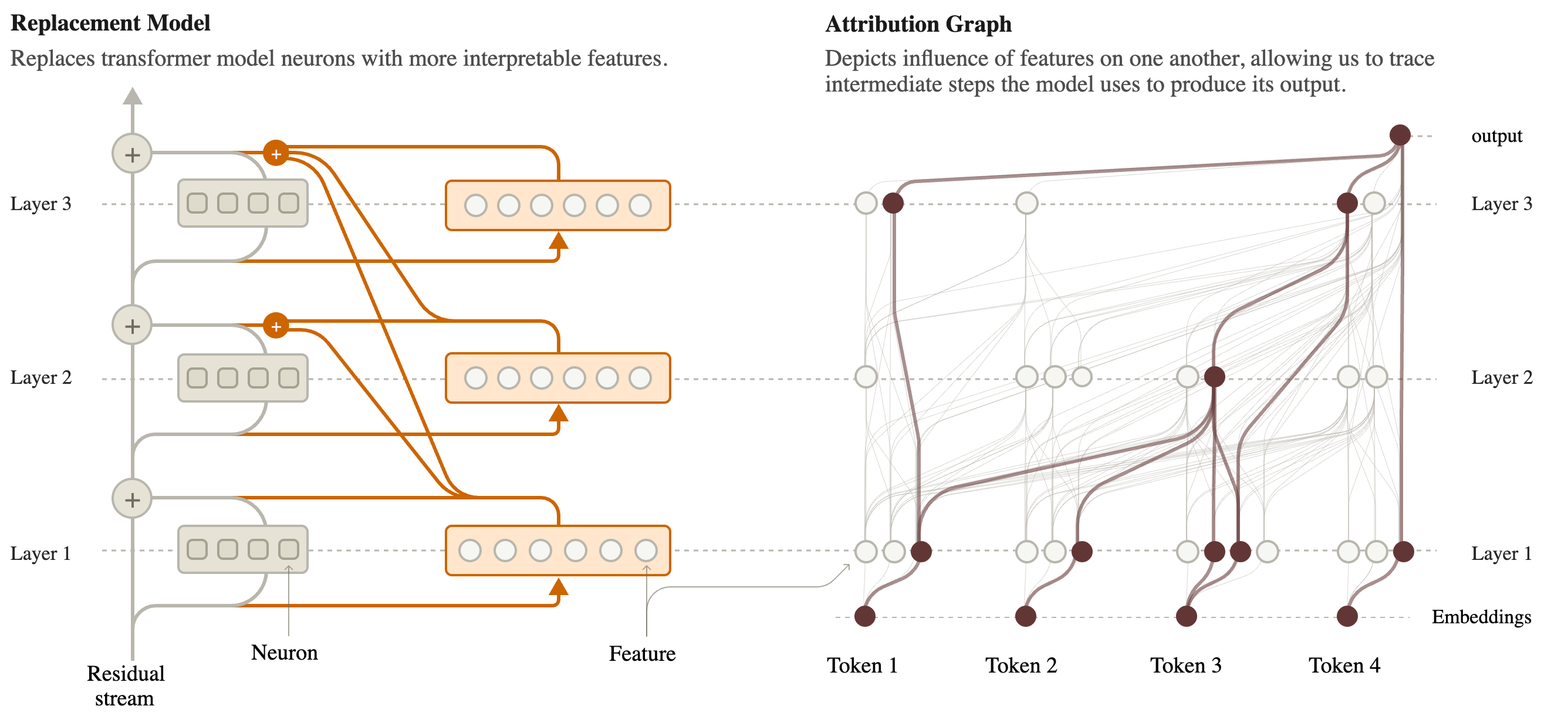{fig-align="center"} **Swap every MLP for a wide layer of sparse features (left). Then trace how features influence one another on a prompt (right).** :::footer Ameisen, E., et al. (2025). [*Circuit Tracing: Revealing Computational Graphs in Language Models*](https://transformer-circuits.pub/2025/attribution-graphs/methods.html). Transformer Circuits Thread. ::: ::: {.notes} The overview figure of the Circuit Tracing paper. Left: the original model has a residual stream going up the middle and an MLP at each layer, drawn as gray boxes of neurons. The replacement puts a set of features, the orange boxes, in place of each MLP. A feature reads from the residual stream at its layer. The orange lines fan out upward: a feature writes to the output of its own layer and to every later layer. That is the 'cross-layer' in cross-layer transcoder. The reason is practical: a concept that persists through many layers is then one feature instead of a chain of copies, which keeps the graphs short. Right: with features as the units, you can ask which features feed which, for a specific prompt. Columns are token positions, rows are layers. That picture is an attribution graph, and the next section is about building and reading it. ::: ## How good is the replacement? :::: {.columns} ::: {.column width="50%"} **Size** * For Claude 3.5 Haiku: **30 million features** across all layers * On average about **235 active** per token position (88 in the smaller 18-layer research model) **Fidelity** * The features miss part of each MLP's output: about **22% normalized error** on Haiku, about 11.5% on the 18-layer model * Run on its own, the replacement gives the 18-layer model's top next token in about **50%** of cases ::: ::: {.column width="50%"} **So the replacement is an approximation, and a rough one.** The fix, for one prompt at a time: * Add an **error node** at every layer and position holding exactly what the features missed * **Freeze** the attention patterns to what the real model did on this prompt **With both, the replacement reproduces the real model's output on that prompt exactly. What is unexplained is on the page, as error nodes.** ::: :::: :::footer Ameisen, E., et al. (2025). [*Circuit Tracing*](https://transformer-circuits.pub/2025/attribution-graphs/methods.html). Transformer Circuits Thread. ::: ::: {.notes} Numbers from the methods paper, and they are worth saying plainly because the pictures later look very clean. Thirty million features sounds like a lot, and it is still not enough to capture everything the MLPs do. A fifth of the signal is missing on the production model. If you let the replacement model run by itself, errors compound from layer to layer and half the time it does not even predict the same next token. The authors' response is a good piece of design. They do not hide the gap. For the one prompt being studied, they compute the difference between the real MLP output and the features' reconstruction and add it back in as a named node. The arithmetic is then exact, and the cost is that some nodes in the graph are labeled 'error' and cannot be interpreted or traced further. They call the result the local replacement model: local because it is only valid for this prompt. ::: # Attribution Graphs ## From the local replacement model to a graph 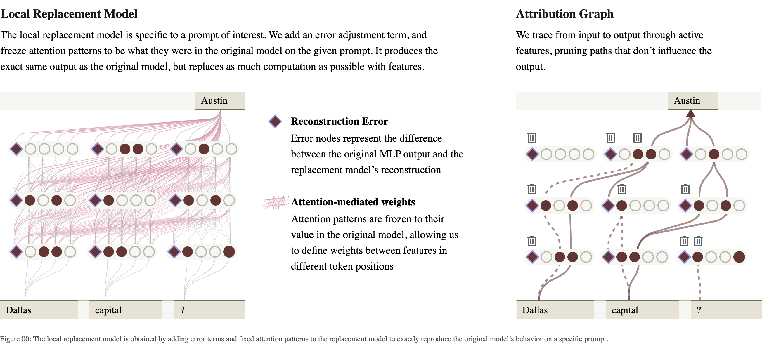{fig-align="center"} **Nodes: active features, input tokens, error nodes (diamonds), and the output. Edges: how much one node contributes to another on this prompt. Then prune.** :::footer Lindsey, J., et al. (2025). [*On the Biology of a Large Language Model*](https://transformer-circuits.pub/2025/attribution-graphs/biology.html). Transformer Circuits Thread. ::: ::: {.notes} Left: the local replacement model for a three-token prompt. Circles are features, filled when active. Diamonds are the error nodes. The pink lines are the frozen attention, which carries information between token positions. Right: the attribution graph. Start at the output token, here 'Austin', and trace backward: which features contributed to it, which features contributed to those, down to the input tokens. Why this is tractable: with attention and normalization frozen, the only nonlinearity left is each feature's own activation. So a feature's input is a sum of contributions from earlier nodes, and each contribution is an edge with a number on it. The raw graph is far too big to read. A short prompt has a couple of hundred active features per token, and the paper notes this produces graphs with millions of edges. Pruning keeps the nodes and edges that matter most for the output. With default settings it removes about nine nodes in ten and keeps about 80 percent of the explained behavior. ::: ## A first graph: completing an acronym :::: {.columns} ::: {.column width="42%"} * Prompt: **The National Digital Analytics Group (N** * The model continues with **DAG** * Read from the bottom: the words *Digital*, *Analytics*, *Group* each activate a feature for their own first letter * "say D" and "say A" combine into "say DA_" * Each box is a **supernode**: several features with the same role, grouped by hand ::: ::: {.column width="58%"} 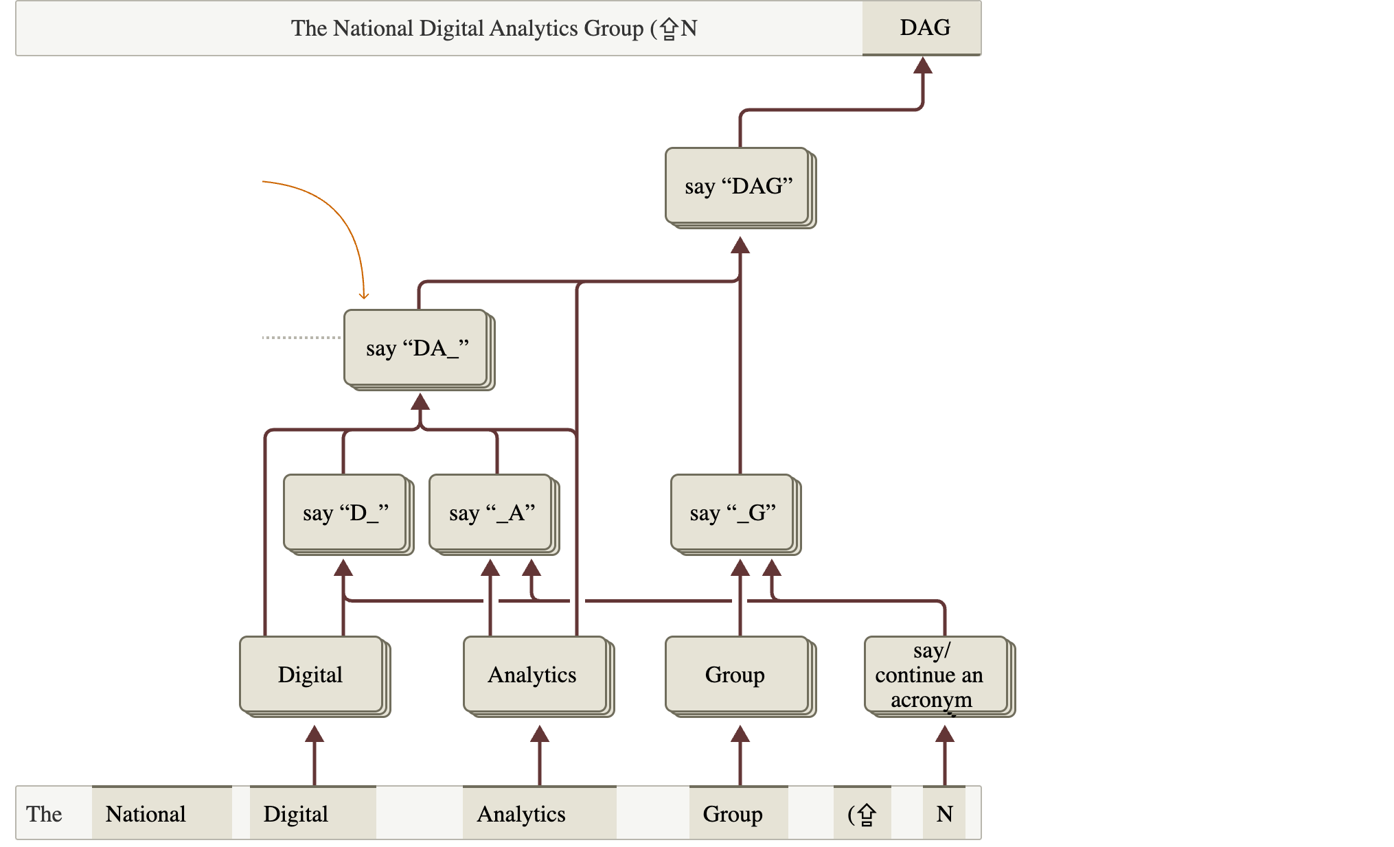{height="760" fig-align="center"} ::: :::: :::footer Ameisen, E., et al. (2025). [*Circuit Tracing*](https://transformer-circuits.pub/2025/attribution-graphs/methods.html). Transformer Circuits Thread. ::: ::: {.notes} The methods paper's worked example, on its 18-layer research model. The organization is made up, so the model cannot have memorized the acronym; it has to compose it. Reading conventions, which every figure from here on shares. Input tokens run along the bottom, the output is at the top right, and arrows point upward from cause to effect. Features sit above the token where they are active. The story the graph tells is small and believable: each word contributes its initial, and the initials are assembled. There is also a 'say or continue an acronym' node on the right, triggered by the open parenthesis and the N. Two caveats that are visible if you look. The boxes are supernodes. The method produces individual features, and a person decided which ones belong together and what to call them. And this is the simplified drawing; the full pruned graph is much larger. ::: ## Is the graph true? Intervene 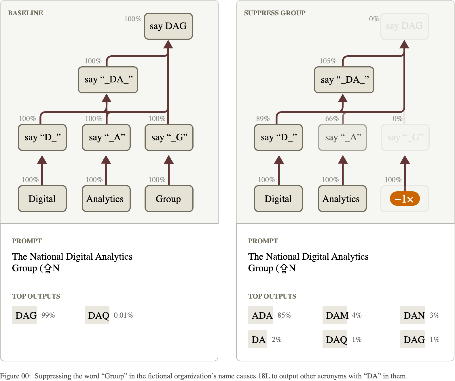{fig-align="center"} **Suppress the "Group" features in the real model. "say G" goes to 0%, and the output changes from DAG to acronyms without the G.** :::footer Ameisen, E., et al. (2025). [*Circuit Tracing*](https://transformer-circuits.pub/2025/attribution-graphs/methods.html). Transformer Circuits Thread. ::: ::: {.notes} A graph drawn from a replacement model is a hypothesis about the real model. This is how it gets tested. Left, baseline: every supernode at 100 percent of its normal activation, and the model says DAG with 99 percent probability. Right: the features in the 'Group' supernode are multiplied by minus one inside the actual model, and the model is run forward. The percentages show what happened downstream. 'say G' drops to zero. 'say A' drops to 66 percent. The top output becomes ADA at 85 percent, and DAG falls to 1 percent. The graph predicted that removing 'Group' should remove the G and leave the D and A. That is what happened. An intervention like this is the difference between a picture that is suggestive and a claim that has been checked. Every case study in the next section comes with one. In visualization terms this is linked views again: a graph on top, and the output distribution it produces underneath. ::: ## Reading a graph is an interface problem :::: {.columns} ::: {.column width="50%"} **What the analyst has to do** * **Label features**: look at the text examples where each one fires most, and at the tokens it pushes the output toward * **Group** features with the same role into supernodes * **Find the path** that matters among many * **Test it** with interventions **How long it takes:** the authors report that the main mechanism can stand out in about ten minutes, and the overall picture takes one to two hours per prompt, before validation. ::: ::: {.column width="50%"} **What the tool gives them** * An interactive graph: hover a node to see its feature, click to pin it, drag nodes, group them * Top inputs and outputs of the selected node, ranked by edge strength * A panel of dataset examples for each feature *"We find that our raw data of attribution graphs is not particularly useful on its own – investing in an ergonomic, interactive interface for exploring them has been essential."* (Lindsey et al., 2025) ::: :::: ::: {.notes} This slide is the link to the rest of the course. The method produces a large labeled graph, and the science happens in a person's head while they explore it. Everything on the right is a technique you know: details on demand, linked views, a ranked list next to a node-link diagram, direct manipulation to arrange and group. The quote is from the discussion section of the Biology paper. The authors list the interface among their main contributions. Everything on the left is manual, and that is a real limitation. Labels are a person's reading of top-activating examples, which is the same procedure that was misleading for neurons. Grouping is subjective. Two analysts could draw different supernodes from the same graph. The papers' pages are interactive: every figure in them can be hovered and opened in the full graph viewer. I recommend opening one after class. ::: # Case Studies ## Two-hop reasoning :::: {.columns} ::: {.column width="32%"} * Prompt: **Fact: the capital of the state containing Dallas is** * Claude 3.5 Haiku answers **Austin** * Does it look up the answer in one step, or go through *Texas*? * The graph: *Dallas* activates **Texas** features; *capital* activates **say a capital**; together they produce **say Austin** * There is also a direct Dallas-to-Austin shortcut. Both paths exist. ::: ::: {.column width="68%"} 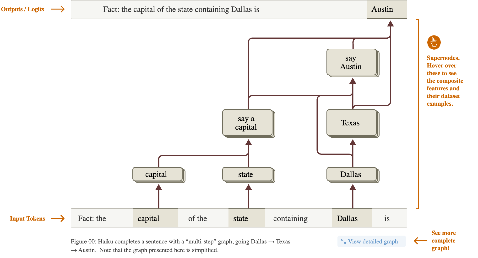{width="100%"} ::: :::: :::footer Lindsey, J., et al. (2025). [*On the Biology of a Large Language Model*](https://transformer-circuits.pub/2025/attribution-graphs/biology.html). Transformer Circuits Thread. ::: ::: {.notes} The introductory example of the Biology paper, now on a production model. The question behind it has been argued about for years: when a model answers a two-step question in one token, did it do two steps internally, or did it memorize the pair? The prompt never mentions Texas. The graph shows an intermediate Texas representation that is caused by 'Dallas' and that in turn helps cause 'say Austin'. So for this prompt there is a real intermediate step. Note what the authors do not claim. They also find direct edges from Dallas to Austin. Both mechanisms run in parallel, and they describe parallel pathways as the rule in everything they looked at. And this is one prompt: an existence proof, in their words, with no claim about how often the model reasons this way. ::: ## Testing it: remove a step 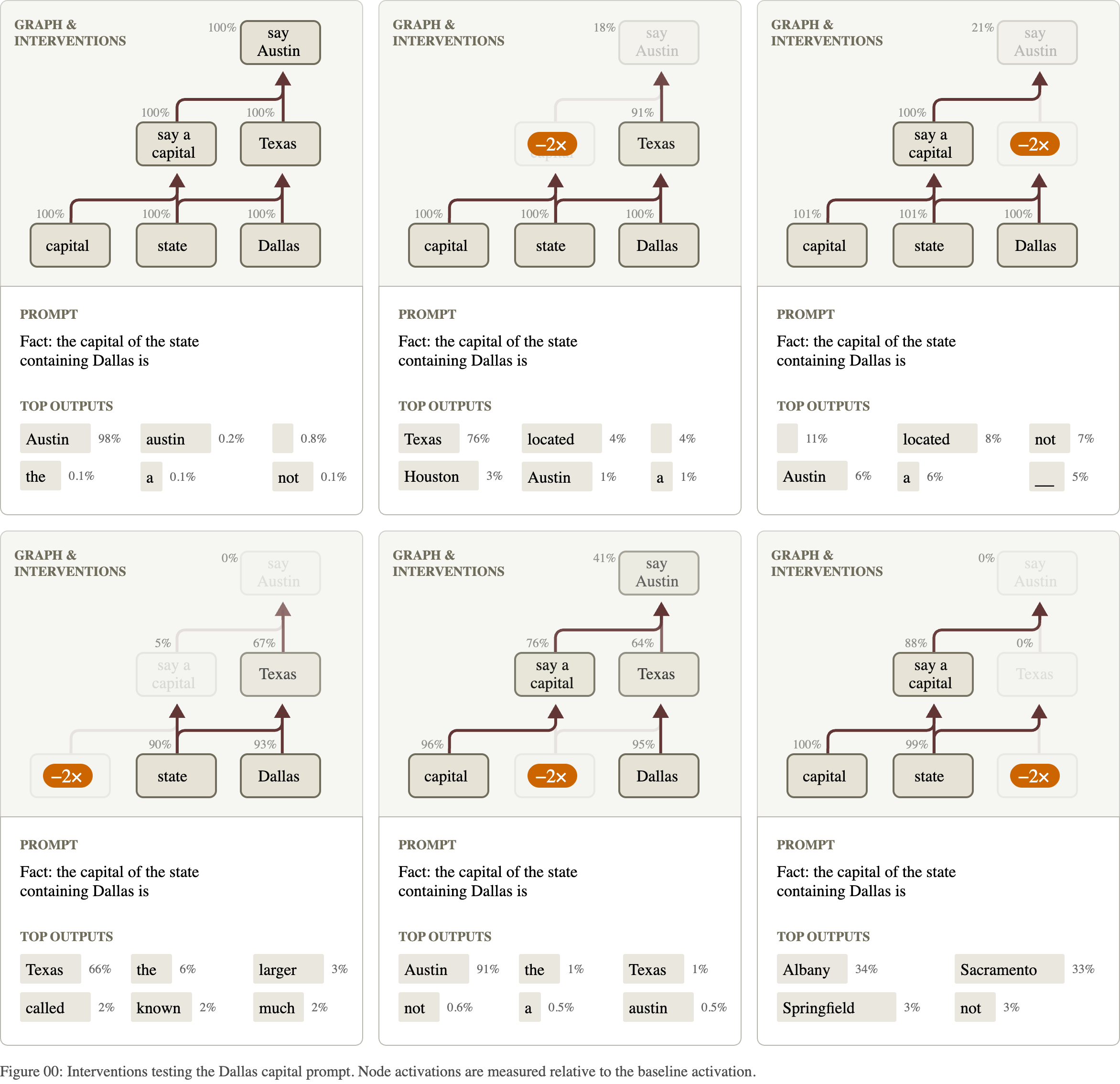{fig-align="center"} **Each panel suppresses one supernode (orange) and shows the effect on the rest and on the top outputs.** :::footer Lindsey, J., et al. (2025). [*On the Biology of a Large Language Model*](https://transformer-circuits.pub/2025/attribution-graphs/biology.html). Transformer Circuits Thread. ::: ::: {.notes} Six small multiples: the baseline at top left and five interventions. Same layout in every panel, so you compare by position. Top left, nothing changed: Austin at 98 percent. Top middle: suppress 'say a capital'. The Texas node is untouched, and the model now says 'Texas': it still knows the state and no longer knows it is supposed to name a capital. Top right: suppress Texas. 'say a capital' is still active, and Austin collapses. The pattern to point out is selectivity. Knocking out one node reduces the nodes downstream of it and leaves the parallel branch alone. That is what the graph's structure predicts, and a diffuse, everything-degrades result would have counted against it. The percentages next to each node are its activation relative to baseline. This figure is a good model for how to present an ablation study: one panel per condition, the manipulated element highlighted, the outcome directly below. ::: ## Testing it: swap the state 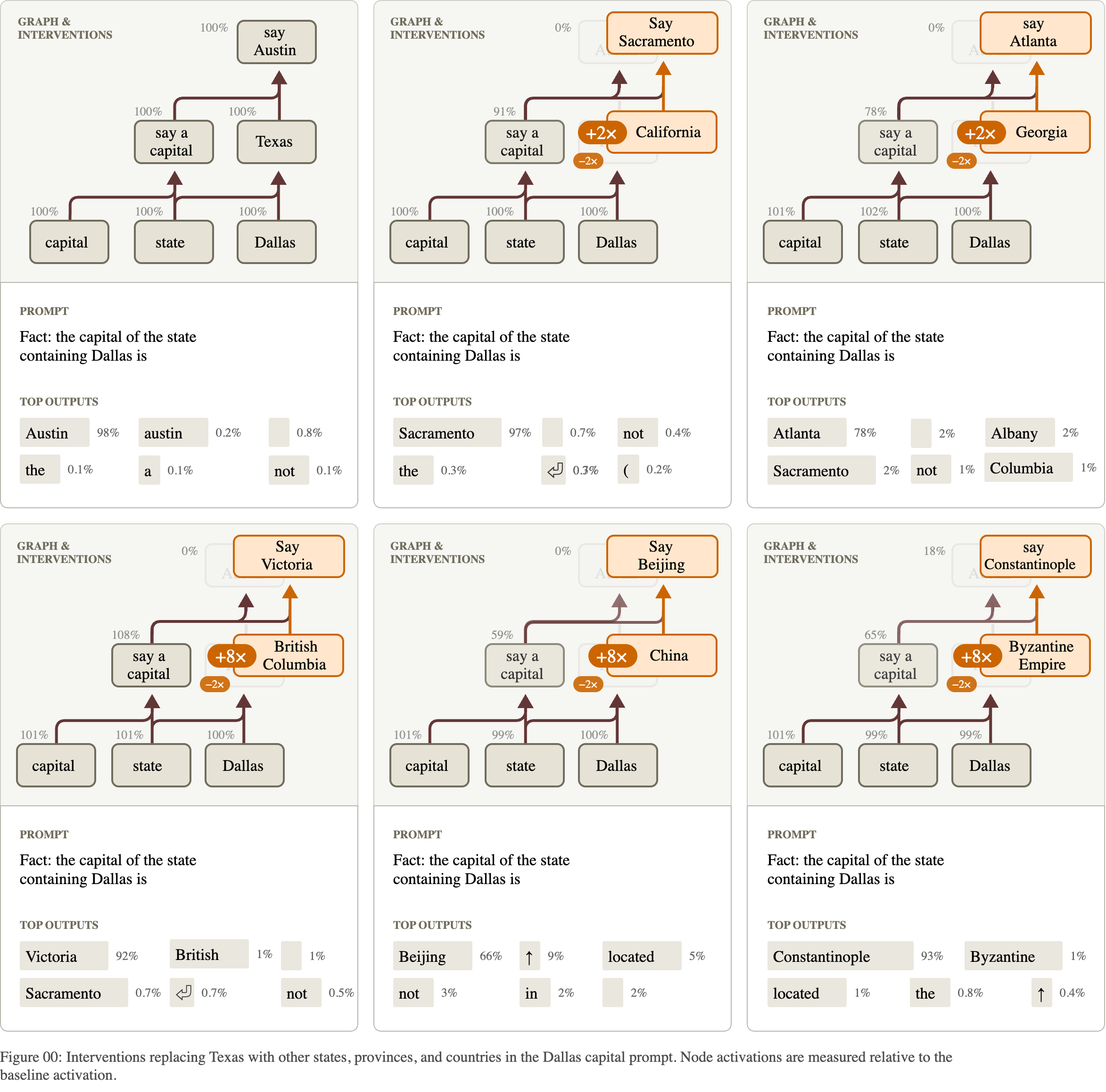{fig-align="center"} **Replace the Texas features with another place's features. The model names that place's capital: Sacramento, Atlanta, Victoria, Beijing.** :::footer Lindsey, J., et al. (2025). [*On the Biology of a Large Language Model*](https://transformer-circuits.pub/2025/attribution-graphs/biology.html). Transformer Circuits Thread. ::: ::: {.notes} A stronger test than deletion. The prompt still says Dallas. The Texas features are suppressed and the features for another region, taken from a different prompt, are added in their place. California in: Sacramento at 97 percent. Georgia: Atlanta at 78. British Columbia: Victoria at 92. China: Beijing. The Byzantine Empire: Constantinople. So the intermediate node is not decoration. It is a variable in the computation, and changing its value changes the answer the way it should. Look at the multipliers in orange. The US states are injected at 2 times their usual strength; the province, the country and the empire need 8 times. The paper says so. The intervention works, and it works less naturally the further the substitute is from what the circuit normally handles. Small numbers like these multipliers are where the honesty of a figure lives. ::: ## Planning in poems :::: {.columns} ::: {.column width="32%"} * Prompt, a rhyming couplet: *He saw a carrot and had to grab it,* * Haiku writes: *His hunger was like a starving rabbit* * Two ways to do this: improvise word by word and find a rhyme at the end, or **pick the rhyme first** * The graph: at the **line break**, before the second line starts, features for **rabbit** and **habit** are already active ::: ::: {.column width="68%"} 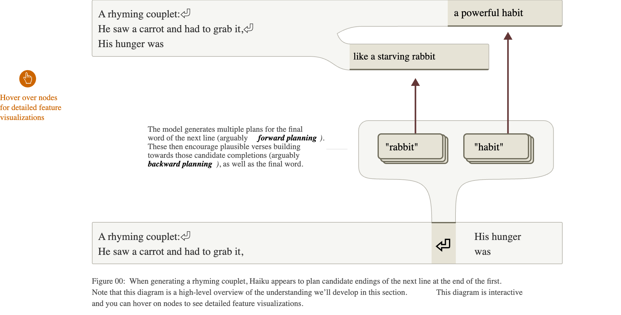{width="100%"} ::: :::: :::footer Lindsey, J., et al. (2025). [*On the Biology of a Large Language Model*](https://transformer-circuits.pub/2025/attribution-graphs/biology.html). Transformer Circuits Thread. ::: ::: {.notes} The result that got the most attention, and the authors say it surprised them. They went in expecting improvisation. The model generates one token at a time. The natural guess is that it writes the line and only at the last word looks for something that rhymes with 'grab it'. The graph says otherwise for this poem. On the newline token at the end of the first line, features for candidate final words are active: rabbit and habit. They then influence the words in between, so the line is written to arrive at the chosen word. The paper calls the first part forward planning and the second backward planning. It is one of the clearest examples of the model representing something about its own future output. Scope, again from the paper: they found planned-word features in about half of the poems they examined. ::: ## Changing the plan 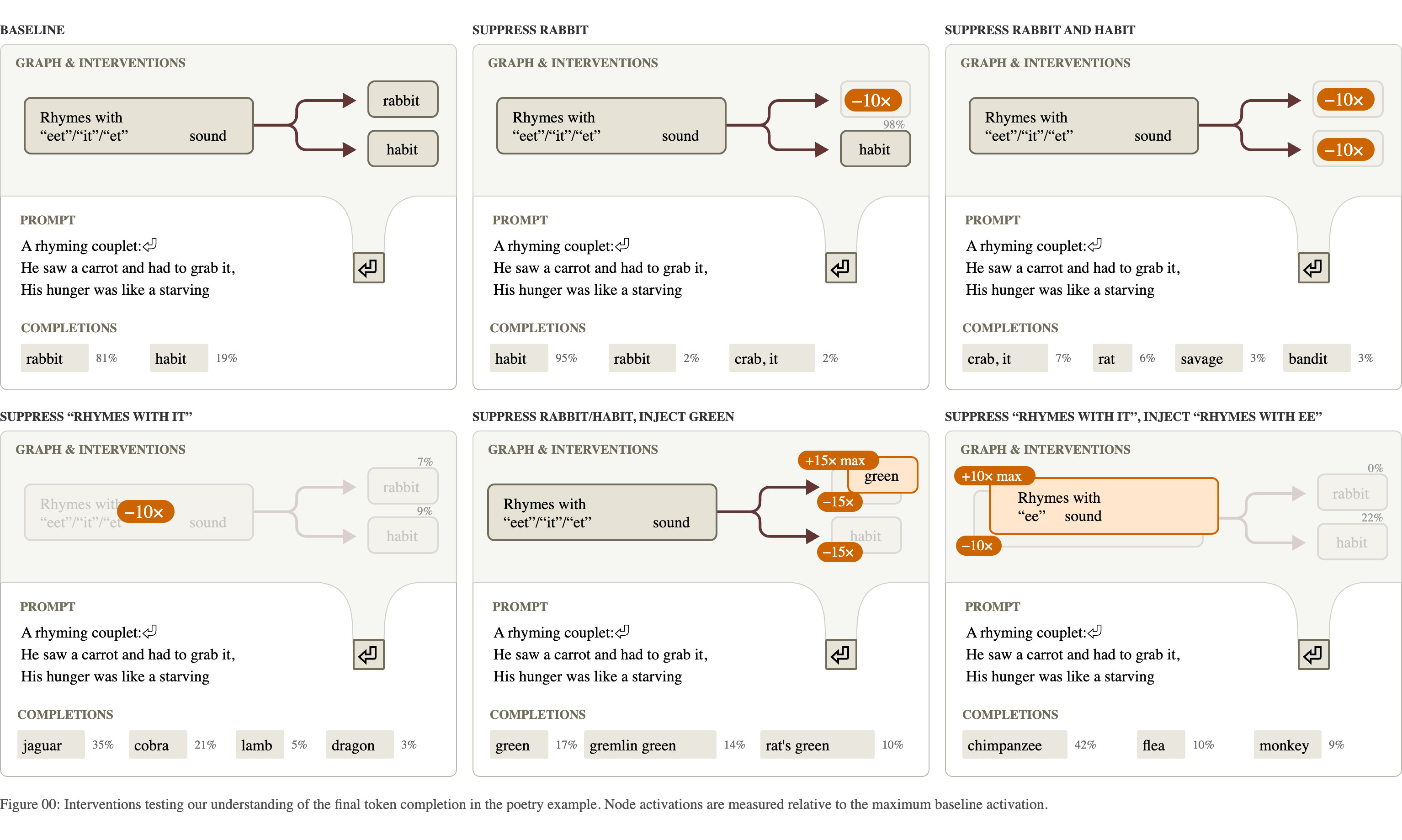{fig-align="center"} **Suppress "rabbit" at the line break and the line ends in "habit". Inject "green" and the model writes a line that ends in "green".** :::footer Lindsey, J., et al. (2025). [*On the Biology of a Large Language Model*](https://transformer-circuits.pub/2025/attribution-graphs/biology.html). Transformer Circuits Thread. ::: ::: {.notes} Six conditions, with the intervention applied only at the newline token and the model then left to write the whole second line. Top left, baseline: rabbit most of the time, habit sometimes. Top middle: suppress the rabbit features. Habit takes over. Top right: suppress both. The model finds other rhymes: 'crab it', 'rat', 'bandit'. Bottom middle: suppress both and inject a feature for the word 'green', which does not rhyme. The line now ends in 'green'. What makes this evidence of planning is that the intervention is at one position and the effect is on a word several tokens later, with the words in between rewritten to lead up to it. In a follow-up on 25 other poems, injecting a planned word made the line end with that word in 70 percent of cases. ::: ## One concept, three languages :::: {.columns} ::: {.column width="32%"} * Prompts: *The opposite of "small" is* in English, French and Chinese * The middle of the graph is shared: **small**, **antonym**, **large** features that do not depend on the language * Language-specific features sit at the two ends: reading the input, and choosing the output word * Three swaps, three predictable changes: the operation, the operand, the output language ::: ::: {.column width="68%"} 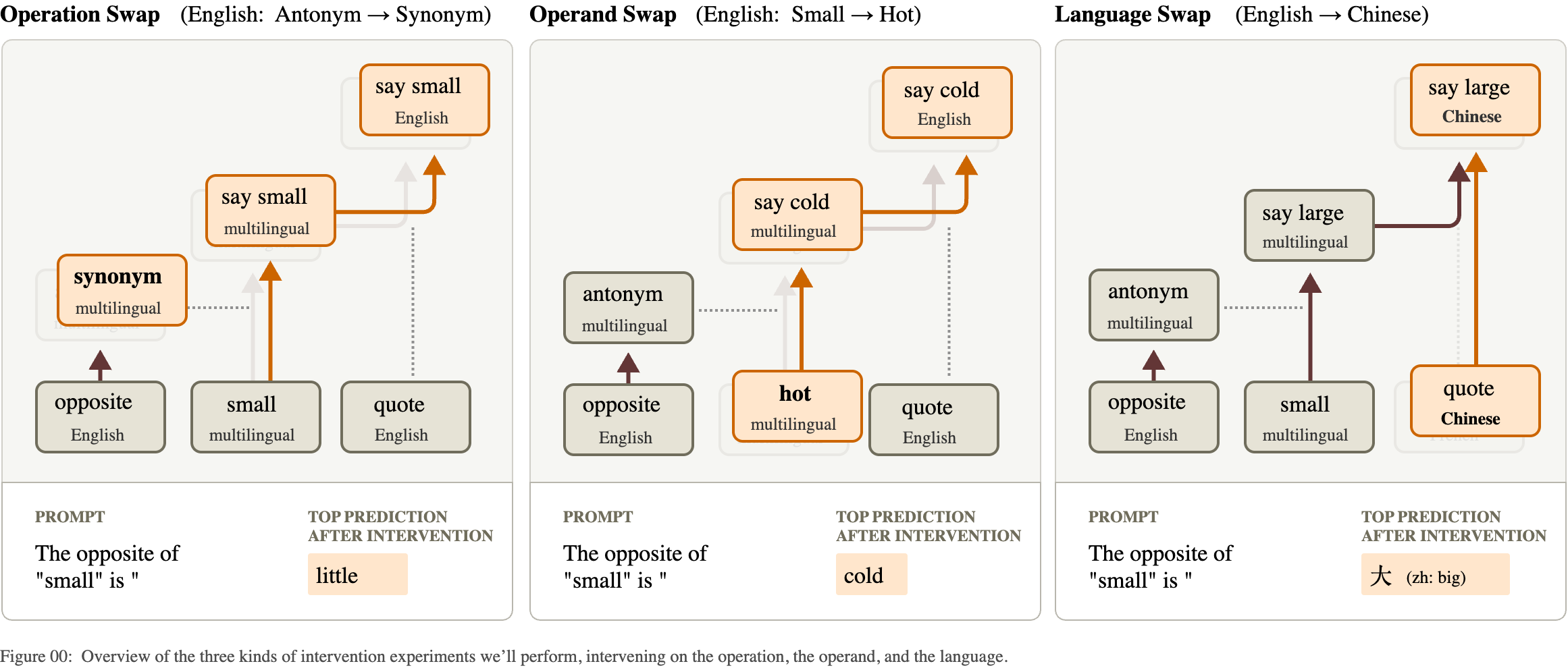{width="100%"} ::: :::: :::footer Lindsey, J., et al. (2025). [*On the Biology of a Large Language Model*](https://transformer-circuits.pub/2025/attribution-graphs/biology.html). Transformer Circuits Thread. ::: ::: {.notes} Does a multilingual model have a separate circuit per language, or one shared one? For this prompt, mostly shared. The figure shows three interventions on the English prompt, each replacing one ingredient. Left: swap the operation from antonym to synonym. The output changes from 'big' to 'little'. Middle: swap the operand from small to hot. The output becomes 'cold'. Right: swap the language feature from English to Chinese. The output is the Chinese word for big. Three independent dials, each doing what its label says. The paper also measures how much of the feature set is shared across languages and finds the share is highest in the middle layers, and higher in this model than in a smaller one. ::: ## Addition, and what the model says about it :::: {.columns} ::: {.column width="50%"} **What the graph shows for 36 + 59** * Several paths in parallel * A **rough-magnitude** path: "about 36 plus about 60 is about 90-something" * A **ones-digit** path: a lookup feature for "ends in 6, plus ends in 9, ends in 5" * The two are combined to give **95** * The same lookup features fire in other contexts that need the sum, such as a citation's year ::: ::: {.column width="50%"} **What the model says when asked how it did it** > "I added the ones (6+9=15), carried the 1, then added the tens (3+5+1=9), resulting in 95." **The explanation is the schoolbook algorithm. The graph shows a different mechanism.** The model's account of its own reasoning is one more output. It can be checked against the mechanism, and here it does not match. ::: :::: :::footer Lindsey, J., et al. (2025). [*On the Biology of a Large Language Model*](https://transformer-circuits.pub/2025/attribution-graphs/biology.html). Transformer Circuits Thread. ::: ::: {.notes} No figure here, because the paper's diagram depends on interactive plots that do not survive as a still image. The structure is simple to state. The model does not carry. It runs approximate and exact computations side by side: one set of features tracks the size of the answer with low precision, and another works out the last digit from the last digits of the operands, using what the authors call lookup-table features. The answer is the number of about the right size that ends in the right digit. Then the authors ask the model how it got 95, and it describes carrying the one. The quote is the model's answer as printed in the paper. This is the cleanest example in the lecture of why level 3 matters. An LLM's explanation of itself is generated the same way as everything else it says: it is what an explanation would plausibly look like. It is not a readout of the computation. ::: ## Hallucination: "I don't know" is the default :::: {.columns} ::: {.column width="45%"} 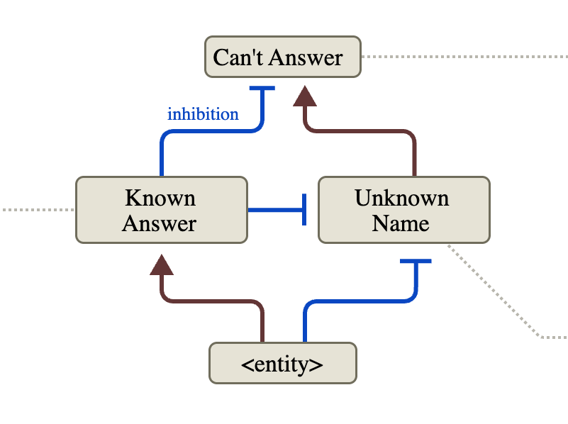{width="100%"} ::: ::: {.column width="55%"} * Ask about a person and a **can't answer** pathway is on **by default** * A name the model recognizes activates **known answer** features * Those **inhibit** the default (blue, T-shaped ends), and the model answers * *Michael Jordan*: known, so it answers "basketball" * *Michael Batkin* (made up): unknown, so it declines **A hallucination, on this account, is the "known" signal firing when the knowledge is not there.** ::: :::: :::footer Lindsey, J., et al. (2025). [*On the Biology of a Large Language Model*](https://transformer-circuits.pub/2025/attribution-graphs/biology.html). Transformer Circuits Thread. ::: ::: {.notes} A summary diagram from the paper. Brown arrows excite, blue T-bars inhibit. The finding is the direction of the default. One might have guessed the model answers unless something tells it to stop. For questions about people it is the other way around: 'can't answer' and 'unknown name' are active by default in the assistant setting, and recognizing the entity switches them off. The base model, without the assistant framing, behaves differently: given 'Michael Batkin plays the sport of' it simply continues with 'Pickleball'. Declining is something the assistant was trained to do, and this circuit is how. That framing makes hallucination a specific failure: familiarity without knowledge. The next two slides test it. ::: ## Turning the circuit by hand 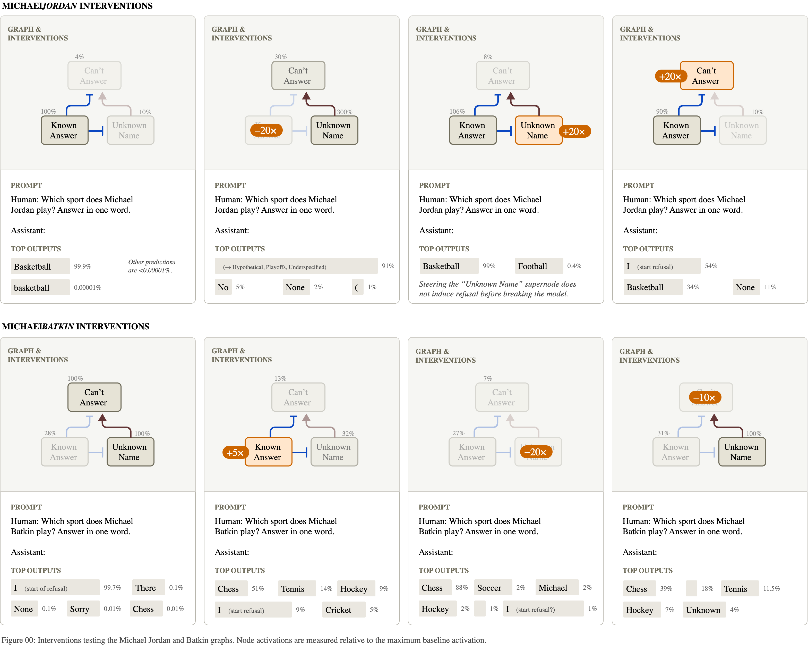{fig-align="center"} **Top: make the model doubt Michael Jordan. Bottom: make it "recognize" Michael Batkin, and it names a sport for a person who does not exist.** :::footer Lindsey, J., et al. (2025). [*On the Biology of a Large Language Model*](https://transformer-circuits.pub/2025/attribution-graphs/biology.html). Transformer Circuits Thread. ::: ::: {.notes} Eight panels: four interventions on the Jordan prompt in the top row, four on the Batkin prompt below. Top left, Jordan baseline: Basketball, near certain. Next to it, suppress the 'known answer' features: the model starts hedging about a hypothetical or unspecified person. At the far right, push 'can't answer' up directly and it begins to refuse. Bottom left, Batkin baseline: the model starts a refusal. Next to it, switch 'known answer' on: it now offers Chess, Tennis, Hockey. That is an induced hallucination, produced by turning on a feeling of familiarity. Suppressing 'unknown name' or 'can't answer' has a similar effect. One panel to be straight about: the third in the top row. Turning up 'unknown name' on the Jordan prompt did not produce a refusal until the intervention was strong enough to break the model, and the figure says so in its caption. The authors report it as a case where the graph's prediction failed. ::: ## A hallucination in the wild {fig-align="center"} **"Name one paper written by Andrej Karpathy." The name is familiar, so the default is suppressed, and the model names a paper he did not write.** :::footer Lindsey, J., et al. (2025). [*On the Biology of a Large Language Model*](https://transformer-circuits.pub/2025/attribution-graphs/biology.html). Transformer Circuits Thread. ::: ::: {.notes} The same circuit, on an error the model makes without any help. Left, unmodified: the model attributes the AlexNet paper to Andrej Karpathy. It is by Krizhevsky, Sutskever and Hinton. In the graph the 'can't answer' node is nearly off: the model knows the name well enough to suppress the default, and does not know his papers well enough to name one. Middle and right: suppress the 'known answer' features by increasing amounts. 'Can't answer' comes back, and the model first gives a hedged, different answer and then, at the stronger setting, apologizes and declines. The paper's control: ask the same question about one of the authors, a much less famous name, and the model declines unprompted. The practical reading is that a model is most likely to make things up about subjects it half knows. ::: ## Chain of thought: is the written reasoning the real reasoning? {fig-align="center"} **Left: the written steps match the computation. Middle: a claimed calculation with nothing behind it. Right: the steps are built backward from the answer the user suggested.** :::footer Lindsey, J., et al. (2025). [*On the Biology of a Large Language Model*](https://transformer-circuits.pub/2025/attribution-graphs/biology.html). Transformer Circuits Thread. ::: ::: {.notes} When a model 'thinks step by step', the steps are text. Whether they describe the computation is an empirical question, and this figure answers it for three cases. Left, faithful: the model has to compute the square root of 0.64. The graph contains a real square-root step on 64, giving 8. What it wrote is what it did. Middle, which the authors call bullshitting in the philosopher Harry Frankfurt's sense: it is asked for the cosine of 23423, which it cannot compute. It writes that it used a calculator and states a value. The graph shows no computation behind the number. It is a guess presented as a result. Right, motivated reasoning: the same question, and the user adds that they worked it out by hand and got 4. The graph shows the model taking the 4 from the hint, dividing by the 5 it knows it will multiply by, and writing 0.8 as the cosine. It worked backward from the answer the user wanted, and the text presents this as working forward. The authors varied the hinted answer, and the written 'derivation' followed the hint each time. They also say the example is artificial and that they knew what to look for. ::: # Attention ## What attribution graphs do not explain {fig-align="center"} **The attention patterns were frozen. The graph shows that information moved from one token to another (left), and cannot show why the model looked there (right).** :::footer Ameisen, E., et al. (2025). [*Circuit Tracing*](https://transformer-circuits.pub/2025/attribution-graphs/methods.html). Transformer Circuits Thread. ::: ::: {.notes} The first item in the methods paper's limitations section, with the authors' own illustration. The prompt is a repeated name: 'Aunt Sally' appears early, and later the text says 'Aunt' again. The model predicts 'Sally' by looking back at what followed 'Aunt' the first time. This is called induction, and it is one of the best understood attention circuits. Left is what the attribution graph shows for it: an edge from the earlier 'Sally' to the output. True, and nearly empty. Right is the actual mechanism, which is all in how the attention pattern is computed: one head notes that the token before 'Sally' was 'Aunt', and another matches the current 'Aunt' against that note. Because the method takes attention patterns as given, any behavior whose interesting part is deciding where to look comes out as a single uninformative arrow. The paper's other example is a multiple-choice question: the graph shows the model attending to option B, and cannot say how it decided B was correct. ::: ## Filter heads {fig-align="center"} **A head that attends to the list item matching a condition. Move its query vector from a "find the fruit" prompt into a "find the vehicle" prompt, and it attends to the fruit.** :::footer Sen Sharma, A., Rogers, G., Shapira, N., & Bau, D. (2025). [*LLMs Process Lists With General Filter Heads*](https://filter.baulab.info/). arXiv:2510.26784. ::: ::: {.notes} A different group, a different model (Llama with 70 billion parameters, 80 layers), and a method aimed at exactly the gap on the previous slide. The task is filtering: here is a list, find the fruit. The authors find attention heads whose attention, from the final token, lands on the item that satisfies the condition. Panel b: the head looks at 'Cherry'. The experiment is activation patching. An attention head compares a query vector, from the token doing the looking, with key vectors from the tokens being looked at. Take the query vector from the fruit prompt, panel a, and insert it into the same head while the model reads a different prompt that asks for a vehicle, panel c. Panel e, unpatched: the head attends to 'Scooter' and the model answers Scooter. Panel f, patched: it attends to 'Peach' and the model answers Peach. So the query vector carries the condition, 'is a fruit', in a form that is independent of the particular list. Panel g is a heat map of heads by layer: the ones with a strong effect are few, and sit in the middle layers. ::: ## The condition is portable 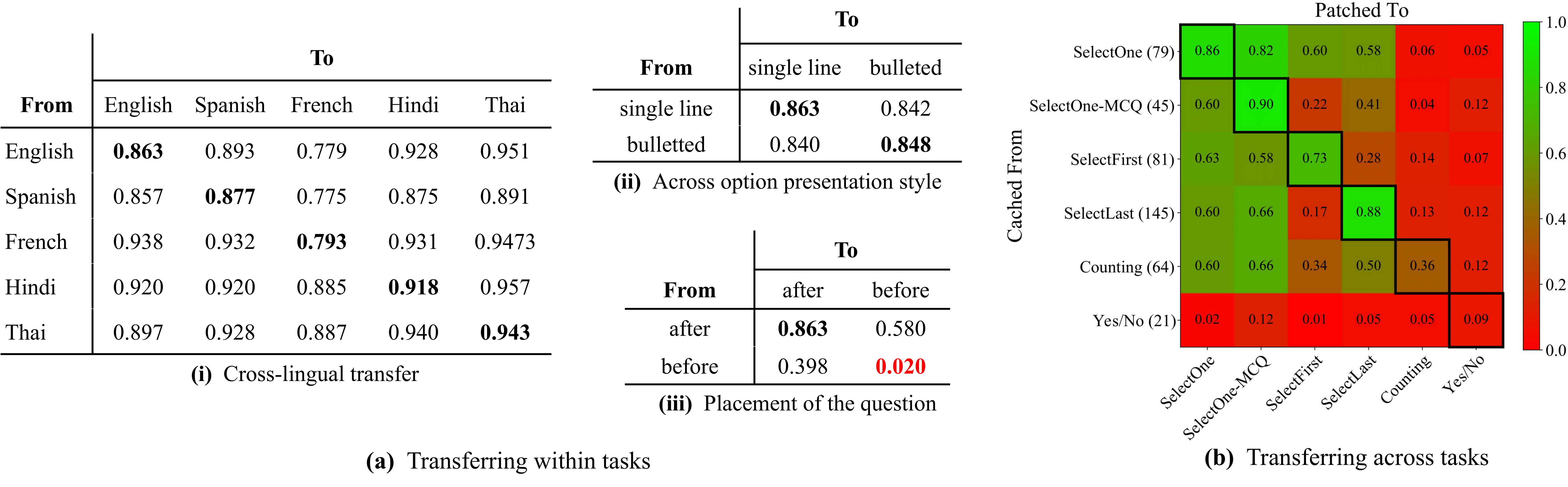{fig-align="center"} **Share of cases in which the patched model answers by the transplanted condition: about 0.8 to 0.95 across languages and list formats, and lower across different tasks.** :::footer Sen Sharma, A., Rogers, G., Shapira, N., & Bau, D. (2025). [*LLMs Process Lists With General Filter Heads*](https://filter.baulab.info/). arXiv:2510.26784. ::: ::: {.notes} How general is that representation? The score in every cell is the fraction of patched runs in which the model gave the answer the transplanted condition implies. Left table: take the condition from a prompt in one language and patch it into a prompt in another. English to Thai, 0.95. Hindi to French, 0.89. The lowest entries are still near 0.78. Whatever the head's query encodes, it is not tied to English words. Middle top: single-line list versus bulleted list, about 0.84 to 0.86 in every direction. Right: a heat map across six tasks that all involve filtering followed by a different final step: select one, select the first match, count, and so on. Transfer is strong between the selection tasks and near zero for yes/no questions. So the same sub-circuit is reused by some tasks and not others. As a figure: three tables and a heat map carrying the same kind of number. The heat map on the right is the one you can read at a glance, and the red-green scale is a poor choice for color-blind readers (Week 2). ::: ## Two strategies: lazy and eager 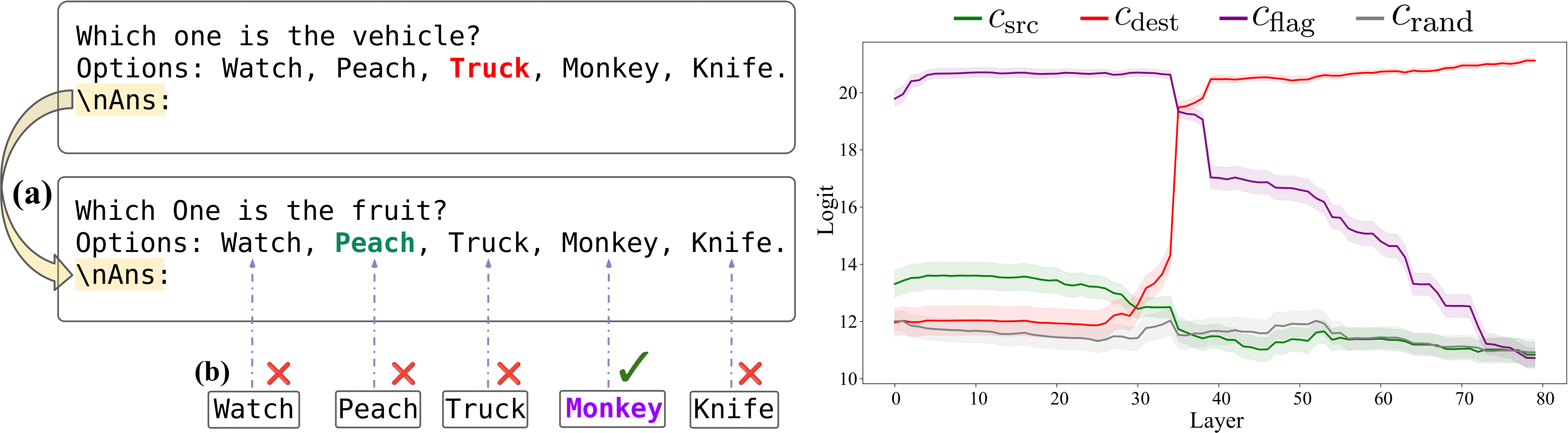{fig-align="center"} **Put the question before the list and the filter heads stop mattering (0.02 on the previous slide). The model marks each item as it reads it.** :::footer Sen Sharma, A., Rogers, G., Shapira, N., & Bau, D. (2025). [*LLMs Process Lists With General Filter Heads*](https://filter.baulab.info/). arXiv:2510.26784. ::: ::: {.notes} Go back to the small table on the previous slide, 'placement of the question'. Question after the list: 0.86. Question before the list, patched into question-before: 0.02. The same task, reordered, and the mechanism is gone. The explanation: when the question comes last, the model cannot know what to look for while reading the items, so it filters at the end using the filter heads. The authors call that lazy evaluation. When the question comes first, the model can judge each item as it arrives and store a marker, a flag, on the ones that match. That is eager evaluation. This figure tests the flag idea. Take the stored state from the item that matched in one prompt and move it onto an unrelated item, 'Monkey', in another. The plot shows, by layer, which answer the model then prefers. Patched at early and middle layers, the purple line is on top: the model picks the item carrying the flag, even though a monkey is neither a fruit nor a vehicle. The lesson for interpretability generally: a mechanism found on one prompt format can fail to exist on a trivially different one. Both papers are careful to say that their findings are about specific prompts. ::: # Limits ## What these pictures can and cannot claim :::: {.columns} ::: {.column width="50%"} **Stated by the authors** * Graphs gave "satisfying insight" for **about a quarter** of the prompts they tried * Each graph is about **one prompt and one output token**: an existence proof * **Error nodes**: part of the computation is unexplained, and more so on long or unusual prompts * **Attention** patterns are taken as given * Features that are **inactive**, and why, do not appear * The replacement may compute the right output by a **different mechanism** than the real MLP ::: ::: {.column width="50%"} **Added by the way the figures are made** * **Feature labels** are a person's reading of top examples * **Supernodes** are grouped by hand * The published cases are the ones that **worked** * Diagrams are **simplified** from pruned graphs, which are pruned from the full graph **What keeps it honest: interventions on the real model, including the ones that failed.** ::: :::: :::footer Lindsey, J., et al. (2025). [*On the Biology of a Large Language Model*](https://transformer-circuits.pub/2025/attribution-graphs/biology.html); Ameisen, E., et al. (2025). [*Circuit Tracing*](https://transformer-circuits.pub/2025/attribution-graphs/methods.html). ::: ::: {.notes} The left column is from the limitations sections of the two papers, which are long and specific. The 'quarter of prompts' figure is from the Biology paper's introduction, with the remark that it is hard to quantify precisely. The right column is what a visualization course should add. Between the model and the figure on the slide there are four reductions: features approximate the MLPs, pruning drops nine nodes in ten, a person groups and labels what is left, and an illustrator simplifies it. Each step makes the picture easier to read and adds a place where a judgment call entered. None of this means the results are wrong. It means the figure is the end of an argument, and the argument's strength is in the interventions. When you read work like this, look for the experiment that could have come out the other way. The authors' own summary of where this stands: a stepping stone, not yet a tool that could certify a model is safe, because a clean graph cannot rule out a mechanism the method failed to see. ::: ## A checklist for reading an interpretability figure 1. **What is the unit?** Neuron, attention head, learned feature, or a hand-made group of features? 2. **Who named it, and from what evidence?** Top-activating examples only, or also its effect on the output? 3. **What is the scope?** One prompt, a family of prompts, or the whole input distribution? 4. **How much is left out?** Reconstruction error, pruned nodes, frozen components. 5. **Is it causal?** Was something changed inside the model, and did the output change as predicted? 6. **What would have counted against it?** Are failed predictions reported? 7. **Does it survive rephrasing?** Remember the question placed before the list. **The same seven questions apply to a saliency map, a SHAP plot or an attention map.** ::: {.notes} A takeaway you can use on any paper in this area, and on your own project figures. Run today's examples through it. The Dallas graph: unit is a hand-made group of learned features; named from top examples and output effects; scope is one prompt; error nodes and pruning acknowledged; causal, with ablations and swaps; the stronger multipliers for non-US regions are a visible weak spot; rephrasing not tested in what we saw. The filter heads: unit is an attention head, which needs no naming; scope is a task family with a measured success rate; causal by construction; and question 7 is exactly where it breaks, which the authors report as a finding. Then run the tools from earlier in the course through it. A SHAP plot does well on scope and poorly on question 5: it is an attribution, with no intervention inside the model. ::: ## What to take away * **Neurons are the wrong unit.** Networks store more features than they have dimensions, as almost-orthogonal directions, when features are sparse. * **Features can be recovered** by dictionary learning, approximately, and the approximation error should be shown. * **An attribution graph** is one prompt's computation drawn in those features, pruned and grouped by a person. * **Inside one production model**, for specific prompts: intermediate reasoning steps, plans made in advance, a default of "I don't know", and explanations that do not match the mechanism. * **Attention needs its own tools**, and patching shows a reusable "filter" operation that depends on how the prompt is ordered. * **A picture of a mechanism is a hypothesis.** The intervention is the evidence. ::: {.notes} One line per part of the lecture. If you remember one thing about method: an explanation of a model should come with an experiment in which the explanation could have failed. If you remember one thing about visualization: the interface is part of the science here. The graphs are unreadable without pruning, grouping, hovering and linked examples, and the choices made in those steps shape what gets found. For the final report: if your project explains a model's behavior, say which of the three levels your explanation is at, and what you did to test it. ::: ## References ::: {.smaller} * Elhage, N., Hume, T., Olsson, C., Schiefer, N., et al. (2022). [*Toy Models of Superposition*](https://transformer-circuits.pub/2022/toy_model/index.html). Transformer Circuits Thread. * Ameisen, E., Lindsey, J., Pearce, A., Gurnee, W., et al. (2025). [*Circuit Tracing: Revealing Computational Graphs in Language Models*](https://transformer-circuits.pub/2025/attribution-graphs/methods.html). Transformer Circuits Thread. * Lindsey, J., Gurnee, W., Ameisen, E., Chen, B., et al. (2025). [*On the Biology of a Large Language Model*](https://transformer-circuits.pub/2025/attribution-graphs/biology.html). Transformer Circuits Thread. * Sen Sharma, A., Rogers, G., Shapira, N., & Bau, D. (2025). [*LLMs Process Lists With General Filter Heads*](https://arxiv.org/abs/2510.26784). arXiv:2510.26784. Project page: ::: ::: {.notes} All four are free online. The three Transformer Circuits papers are interactive web pages: the figures respond to hovering and link to full graphs. A reading order for someone new to this: the introduction and first two experiments of Toy Models of Superposition, then the Biology paper's introduction and whichever case studies interest you, then the methods paper for how it works. The filter heads project page is short and has interactive attention examples. ::: ## Next: project presentations * **Tuesday, Dec 1 and Tuesday, Dec 8**: final project presentations * **Dec 14**: final project report due (8 pages) ::: {.notes} This was the last regular lecture. The next two Tuesdays are presentations, and the report is due December 14, the week after the last class. Thanksgiving recess is Thursday and Friday of this week and does not affect our Tuesday meetings. :::