# Model Assessment ## Agenda \ 1. Confusion Matrices and ROC Curves 2. Visual Analytics Systems for Model Performance 3. Calibration ::: {.notes} Today we're going to talk about model assessment and evaluation. We'll start with some of the most common tools: confusion matrices and ROC curves. Then we'll look at some more advanced visual analytics systems for evaluating model performance. Finally, we'll do a deep dive into the concept of calibration, which is becoming increasingly important in modern machine learning. ::: # Confusion Matrices, ROC Curves ## Scenario: Disease Prediction * Consider a disease prediction model. Suppose the hypothetical disease has a 5% prevalence in the population * The given model converges on the solution of predicting that nobody has the disease (i.e., the model predicts "0" for every observation) * Our model is 95% accurate * Yet, public health officials are stumped ::: {.notes} This scenario illustrates a common problem with using a single metric like accuracy to evaluate a model, especially with imbalanced datasets. A model can achieve high accuracy by simply predicting the majority class, but it will be useless in practice. This is why we need more sophisticated evaluation methods. Make the numbers concrete. Take 1,000 people: 50 have the disease, 950 do not. The model says "healthy" to everyone. It is right about all 950 healthy people and wrong about all 50 sick ones, so accuracy is 950 out of 1,000, 95 percent. But it finds zero of the 50 patients, so its recall or sensitivity is 0, which for a screening test is the only number that matters. It never predicts "sick", so precision is not even defined. Ask the room: what should the officials have asked for? Two answers. First, a baseline: always compare accuracy with what a constant majority-class guess gets, which here is also 95 percent. This model has learned nothing beyond the prevalence. Second, the errors broken down by type: a missed case and a false alarm have very different costs, and a single accuracy number adds them together. That breakdown is the confusion matrix, coming up shortly. One more point to plant for later: a model like this often still ranks patients sensibly. Its scores may put the sick people higher, but every score falls below the 0.5 cutoff. Then the fault is the threshold, not the model, and the ROC curve is the tool that separates those two things. ::: ## Scenario: Handwritten Digits :::: {.columns} ::: {.column width="55%"} * Consider a model to identify handwritten digits. All digits are equally probable and equally represented in the training and test datasets. * The model correctly identifies all of the digits, except for digit $5$, classifying half of the $5$s samples as $6$ and the other half is correctly identified * The accuracy of this model is $95\%$. Is this information enough to determine whether the model is good or not? ::: ::: {.column width="45%"} 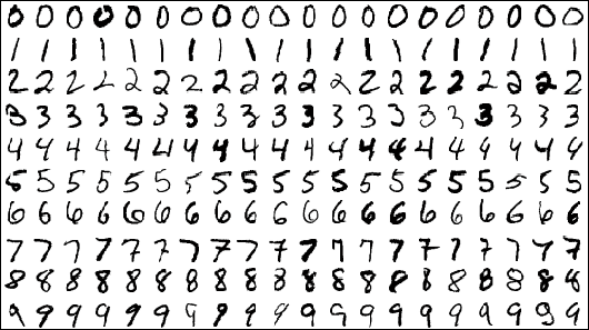{width="100%" fig-align="center"} ::: :::: ::: {.notes} Second way accuracy misleads, and this time imbalance is not the excuse: all ten digits are equally common. Ask the question on the slide and let them answer before going on. Check the arithmetic with them. Each digit is 10 percent of the data. Half of the 5s are wrong, which is 5 percent of all samples, so accuracy is 95 percent. Now picture a second model, also 95 percent accurate, that gets 5 percent of every digit wrong, scattered across all the other classes. On paper the two models are identical. In practice they are not. The first has one systematic blind spot. If it reads ZIP codes or bank cheques, every other 5 turns into a 6, the same way every time, and a user will notice. The second makes rare, unpredictable slips. The fixes differ too. The systematic error points at something specific: more or better 5s in the training data, augmentation, or a look at the 5 against 6 boundary. Diffuse errors point at model capacity or label noise. A single accuracy number cannot tell you which situation you are in. Even per-class averages can hide it. Recall is 100 percent for nine digits and 50 percent for the 5s, so macro-averaged recall is 95 percent again. The problem only shows up when you look at the individual cells: 5s predicted as 6s. The 6 class also pays a price. Its precision drops to about 67 percent, because a third of what the model calls a 6 is really a 5. So what we need is a view of which errors, not how many. That view is the confusion matrix, starting on the next slide. Handwritten digits come back several times today: scikit-learn's 8-by-8 digits in the confusion matrix example, MNIST in Squares, and the UCI pen-based digits in Alsallakh. ::: ## Extended Confusion Matrix 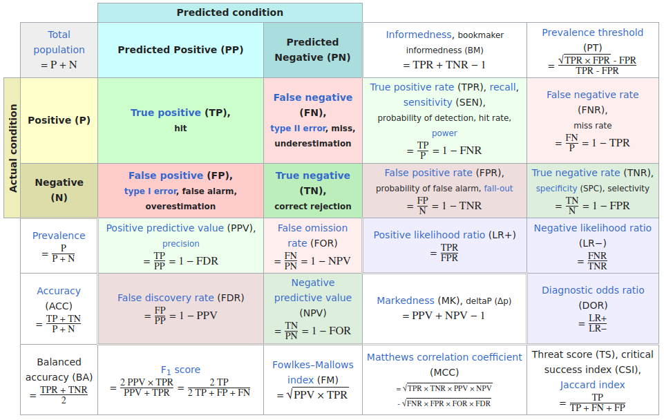{fig-align="center"} ::: footer Table from Wikipedia: [Confusion matrix](https://en.wikipedia.org/wiki/Confusion_matrix) ::: ::: {.notes} Wikipedia's table, and it is worth a minute because the whole first third of the lecture lives in it. The coloured two-by-two in the top left is the confusion matrix: TP, FN, FP, TN. Every other cell on the slide is computed from those four numbers. Point at the four we use today: true positive rate or recall (TP over P) and false positive rate (FP over N) are the two axes of the ROC curve; precision or positive predictive value (TP over predicted positive) and recall are the two axes of the PR curve; accuracy is in the left column, just above balanced accuracy. Note that TPR and FPR each stay within one row, so they do not depend on class balance, while precision mixes the rows and does. That one observation explains the ROC versus PR discussion later. Go back to the disease model and fill in its cells, per 1,000 people: TP 0, FN 50, FP 0, TN 950. Accuracy is 95 percent. TPR is 0. Balanced accuracy, the bottom-left cell, averages TPR and TNR: (0 + 1) / 2, which is 50 percent, exactly chance. Had the officials seen that number, they would not have been stumped. F1 is 0, and precision is 0 over 0, undefined, because the model never predicts positive. Make "precision mixes the rows" concrete with one test used in two populations. Say TPR is 90 percent and FPR is 5 percent. At 50 percent prevalence, per 1,000 people: 450 true positives and 25 false positives, so precision is 95 percent. At 5 percent prevalence: 45 true positives, and 5 percent of 950 negatives, about 48 false positives, so precision is under 50 percent. It is the same classifier with the same ROC point, and half its positive calls are now wrong. This is the base-rate effect behind rare-disease screening, and it is why PR curves change with class balance while ROC curves do not. Last, the names. Each quantity has three or four, one per field, and the table lists them all. Medicine says sensitivity and specificity. Information retrieval says precision and recall. Statistics says power and type I error rate, which is the FPR. Signal detection, where ROC comes from, says hit rate and false alarm rate. Tell them not to memorize the table: know the four cells, and derive everything else when they need it. ::: ## Confusion Matrices: A Deeper Look ::::::: {.columns .smaller} ::: {.column} 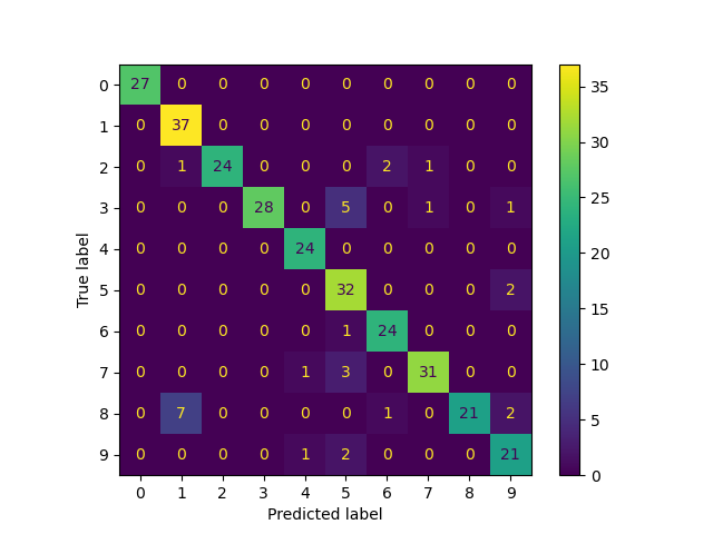{width="100%" fig-align="center"} scikit-learn digits: label spreading trained on 40 labelled images, tested on 300 (accuracy 90%) ::: ::: {.column} **Reading it:** rows are the true label, columns the predicted label. The diagonal is correct. **Pros** - Shows *which* classes are confused, not just how many errors - Precision, recall and F1 for every class can be read off it **Cons** - Scales badly: 100 classes means 10,000 cells - Drops the scores: "barely wrong" and "confidently wrong" count the same - Hides the instances behind each count Squares, Neo and the confusion wheel, later today, each attack one of these. ::: :::: ::: footer [code](https://scikit-learn.org/stable/auto_examples/semi_supervised/plot_label_propagation_digits.html) ::: ::: {.notes} A real ten-class matrix, from a scikit-learn example. The model does not matter much today: it is label spreading, a semi-supervised method, given only 40 labelled digits and scored on 300 others, so it gets about 90 percent. What matters is the reading. Start with the convention. Rows are the true label and columns the predicted label, same as the Wikipedia table. Warn them now: Fawcett's figure in the ROC section puts the true class across the columns. Check the axis labels every time, because the transposed version reads as the opposite story. Read it with them. The diagonal is bright, and the off-diagonal mass sits in a few cells: seven 8s read as 1s, five 3s read as 5s, three 7s read as 5s. That is the 'which errors' view the handwritten-digits slide asked for. Then two readings that need the whole row or column. Along row 8, only 21 of 31 eights are right, so recall for 8 is 68 percent, the worst class. Down column 5, 43 digits were called 5 but only 32 were 5s: 3s, 7s, 9s and a 6 all drain into it, so precision for 5 is 74 percent. Also point out the asymmetry: 8 becomes 1 seven times, and 1 never becomes 8. A confusion matrix is not symmetric, and the direction tells you something. Then the limits, on the right. It does not scale past a few dozen classes. It throws away the scores: a prediction that was barely wrong looks the same as one that was confidently wrong. And it hides the instances, so you cannot click through to the seven offending 8s. Neo answers the scaling problem with hierarchy. Squares and the confusion wheel put the scores back and let you reach the instances. ::: ## Confusion Matrices: Spend the Colour on the Errors :::: {.columns} ::: {.column width="38%"} - Same matrix. The diagonal is now grey: colour is spent only on mistakes - Right margin: **recall** per true class. Bottom margin: **precision** per predicted class - 8 is the weakest class (68% recall); 5 is a sink that absorbs 3s, 7s, 9s and a 6 (74% precision) ::: ::: {.column width="62%"} ```{python} #| echo: false import numpy as np import matplotlib.pyplot as plt from sklearn import datasets from sklearn.semi_supervised import LabelSpreading from sklearn.metrics import confusion_matrix # Reproduces scikit-learn's plot_label_propagation_digits example exactly digits = datasets.load_digits() rng = np.random.RandomState(2) idx = np.arange(len(digits.data)); rng.shuffle(idx) X, y = digits.data[idx[:340]], digits.target[idx[:340]] y_train = y.copy(); y_train[40:] = -1 lp = LabelSpreading(gamma=0.25, max_iter=20).fit(X, y_train) cm = confusion_matrix(y[40:], lp.transduction_[40:], labels=range(10)) errors = np.ma.masked_where(np.eye(10, dtype=bool) | (cm == 0), cm) plt.rcParams.update({'font.size': 17}) fig, ax = plt.subplots(figsize=(10, 9.4)) ax.imshow(np.eye(10), cmap='Greys', vmin=0, vmax=8) # pale grey diagonal ax.imshow(errors, cmap='Oranges', vmin=0, vmax=cm[~np.eye(10, dtype=bool)].max()) for i in range(10): for j in range(10): if i == j: ax.text(j, i, cm[i, j], ha='center', va='center', color='#999999', fontsize=16) elif cm[i, j]: ax.text(j, i, cm[i, j], ha='center', va='center', fontsize=19, weight='bold', color='white' if cm[i, j] > 4 else '#222222') recall = cm.diagonal() / cm.sum(axis=1) precision = cm.diagonal() / cm.sum(axis=0) for i, r in enumerate(recall): ax.text(10.9, i, f'{r*100:.0f}', ha='right', va='center', color='#222222') for j, p_ in enumerate(precision): ax.text(j, 10.2, f'{p_*100:.0f}', ha='center', va='center', color='#222222') ax.text(10.9, -0.95, 'recall %', ha='right', fontsize=15, color='#555555') ax.text(-0.75, 10.2, 'precision %', ha='right', va='center', fontsize=15, color='#555555') ax.set_xticks(range(10)); ax.set_yticks(range(10)) ax.set_xlabel('Predicted label', labelpad=12); ax.set_ylabel('True label') ax.xaxis.set_label_position('top'); ax.xaxis.tick_top() ax.set_xlim(-0.5, 11.0); ax.set_ylim(10.7, -0.5) for side in ax.spines.values(): side.set_visible(False) ax.tick_params(length=0) plt.show() ``` ::: :::: ::: {.notes} SKIPPABLE - if running long, jump to Confusion Matrices in sklearn. A design point from this course, applied to the last slide. In the original, the colour scale runs from 0 to 37, and the diagonal uses almost all of it. Every error is 7 or fewer, so all the errors land in nearly the same dark purple, and the errors are the part we care about. Here the diagonal is taken out of the colour scale and printed in grey. The single-hue orange ramp now covers only the errors, 1 to 7, and the 8-to-1 cell and the 3-to-5 cell stand out immediately. The margins do the arithmetic from the Wikipedia slide for them. Recall is each row's diagonal over the row total; precision is each column's diagonal over the column total. Read the two extremes: 8 has 68 percent recall, it leaks into 1, 6 and 9; 5 has 74 percent precision, everything drains into it. The class sizes differ, from 24 to 37 test digits, so row percentages are fairer than raw counts when comparing classes. The figure is generated live from the same scikit-learn example, so the numbers match the previous slide exactly. This is the idea behind the Alsallakh confusion matrix later: augment the grid with the per-class summaries. ::: ## Confusion Matrices in sklearn ```{python} #| echo: true from sklearn import datasets from sklearn.linear_model import LogisticRegression from sklearn.model_selection import train_test_split X,y = datasets.make_classification(5000, 10, random_state=42) X_train, X_test, y_train, y_test = train_test_split(X, y, random_state=42) clf = LogisticRegression(random_state=0) ``` ```{python} #| echo: true #| output-location: column import matplotlib.pyplot as plt from sklearn.metrics import ConfusionMatrixDisplay clf.fit(X_train, y_train) ConfusionMatrixDisplay.from_estimator(clf, X_test, y_test, cmap=plt.cm.Blues) plt.show() ``` ::: {.notes} The scikit-learn version, and the pattern repeats for every display today: build data, fit, then a Display class with from_estimator. Here it is a synthetic binary problem, 5,000 samples and 10 features, logistic regression. The figure on the right is the live output of the cell on the left, executed when the deck was rendered. Read the matrix: two large diagonal cells, two small off-diagonal ones, roughly balanced errors. The colour ramp is a single-hue sequential scale, the right choice from last week's colour lecture. ::: ## Neo: Hierarchical Confusion Matrix ::: {style="text-align: center;"} ::: ::: footer Görtler, J., Hohman, F., Moritz, D., et al. (2022). [*Neo: Generalizing Confusion Matrix Visualization to Hierarchical and Multi-Output Labels*](../refs/Goertler_Hohman_Moritz_2022_Neo_Confusion_Matrix.pdf). CHI. ::: ::: {.notes} Neo is a research project that introduces a hierarchical confusion matrix. This is particularly useful when you have a large number of classes that have a natural hierarchy. For example, if you are classifying animals, you might have a hierarchy of mammals, birds, reptiles, etc. A hierarchical confusion matrix can help you see if your model is making errors at a high level (e.g., confusing a mammal for a bird) or at a low level (e.g., confusing a cat for a dog). ::: ## Receiver Operating Characteristic (ROC) :::: {.columns} ::: {.column width="60%"} * ROC analysis is another way to assess a classifier's output * ROC analysis developed out of radar operation in the second World War, where operators were interested in detecting signal (enemy aircraft) versus noise * We create an ROC curve by plotting the true positive rate (TPR) against the false positive rate (FPR) at various thresholds * **True Positive Rate (TPR)**, also known as Recall or Sensitivity, is the proportion of actual positives that are correctly identified as such (TP / (TP + FN)). * **False Positive Rate (FPR)** is the proportion of actual negatives that are incorrectly identified as positive (FP / (FP + TN)). ::: ::: {.column width="35%"} 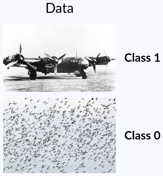{width="100%" fig-align="center"} ::: :::: ::: {.notes} ROC comes out of signal detection theory and wartime radar: an operator looks at a blip and has to decide aircraft or flock of birds, which is exactly the picture on the right, class 1 and class 0. The operator's willingness to say 'aircraft' is a threshold. Lower it and you catch more aircraft and raise more false alarms. The ROC curve is the plot of that trade-off: true positive rate against false positive rate as the threshold sweeps. The name is a leftover from that setting: the 'receiver' is the radar receiver, and the 'operating characteristic' describes how its operator performs across settings. From radar it went into psychology as signal detection theory, then into medicine for judging diagnostic tests (Swets wrote the standard account in Science in 1988), and into machine learning around 1989. That history is why the Wikipedia table had so many names: hit rate and false alarm rate are the radar and psychology words for TPR and FPR. The idea to plant now: a model that outputs a score is not one classifier, it is a family of classifiers, one per threshold. Accuracy, precision and the confusion matrix each describe one member of that family. The ROC curve shows the whole family at once. Picking the threshold is a separate decision, and it depends on costs: a missed bomber is far worse than chasing a flock of geese. Point at the two rates again. TPR uses only the positives and FPR uses only the negatives, each within one row of the confusion matrix. That is why the curve does not move when class balance changes, and also why it can hide what happens to precision. We come back to that at the end of this section. ::: ## ROC Curve :::: {.columns} ::: {.column width="60%"} {width="85%" fig-align="center"} ::: {.fragment} 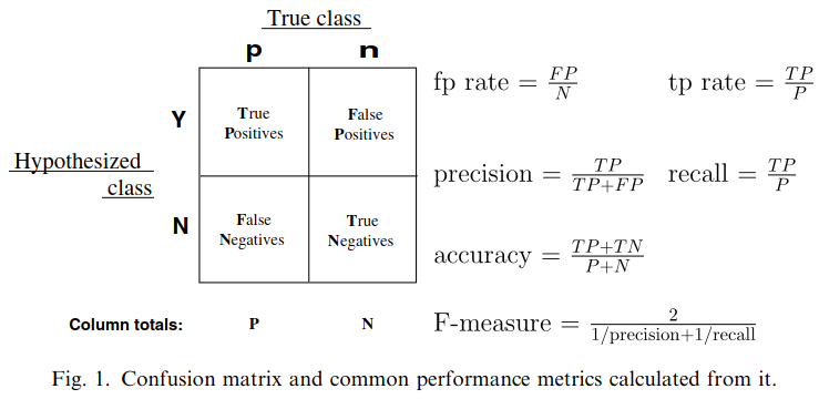{width="85%" fig-align="center"} ::: ::: ::: {.column width="40%"} ::: {.fragment} 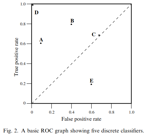{width="100%"} ::: ::: :::: ::: footer Fawcett, T. (2006). [*An introduction to ROC analysis*](../refs/Fawcett_2006_Introduction_ROC_Analysis.pdf). Pattern Recognition Letters, 27(8), 861-874. ::: ::: {.notes} Three figures from Tom Fawcett's 2006 tutorial, which is the reference for this section and is linked in the footer. First his confusion matrix, with the rates written out. Remind them of the warning from the confusion matrix slide: here the true class runs across the columns, the transpose of scikit-learn. Then, on the click, ROC space with five discrete classifiers. A discrete classifier outputs only a label, so it is a single point. Walk through them. D at the top left is perfect. A is what Fawcett calls conservative: it says positive only on strong evidence, so it has few false positives but misses many positives. B is more liberal: it catches more positives and pays with more false alarms. Ask the room whether A or B is better. The honest answer is that it depends on the costs and the class balance, and the graph alone cannot settle it. C sits on the diagonal, which is random guessing. At (0.7, 0.7) it is guessing positive 70 percent of the time: it catches 70 percent of the positives and raises false alarms on 70 percent of the negatives. Moving along the diagonal just changes how often you guess. To get above it, a classifier has to use some information in the data. E is below the diagonal, worse than random, and it is informative. Fawcett points out that E is exactly B negated. Flip every decision and TPR becomes 1 minus TPR, FPR becomes 1 minus FPR, so E's point maps onto B's. A classifier below the diagonal has useful information and applies it backwards. One more remark from the paper worth repeating: when negatives vastly outnumber positives, as they usually do, the interesting part of the graph is the far left, where false positives are rare. A scoring classifier, next slide, traces a whole curve instead of a single point. ::: ## ROC Curve :::: {.columns} ::: {.column width="45%"} 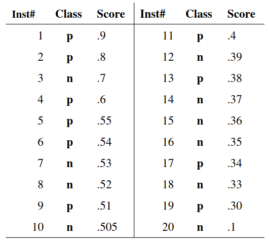{height="700" fig-align="center"} ::: ::: {.column width="55%"} 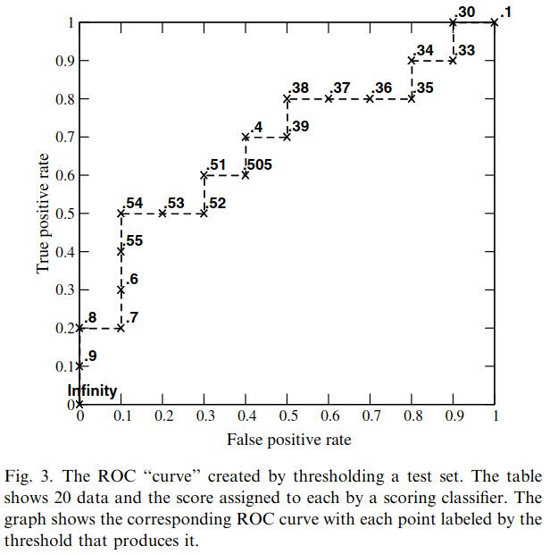{height="760" fig-align="center"} ::: :::: ::: footer Fawcett, T. (2006). [*An introduction to ROC analysis*](../refs/Fawcett_2006_Introduction_ROC_Analysis.pdf). Pattern Recognition Letters, 27(8), 861-874. ::: ::: {.notes} How the curve is built, Fawcett's Figure 3. Left: twenty test instances, ten positive and ten negative, sorted by score. Right: the curve, each point labelled by the threshold that produces it. Build the first steps with them. Start with the threshold above every score: nothing is called positive, so we are at the origin, (0, 0). Lower the threshold past each instance in turn: if it is a positive, step up; if it is a negative, step right. With ten of each, every step is 0.1. At 0.9 the first instance, a positive, is called positive, so we are at (0, 0.1). At 0.8, another positive: (0, 0.2). At 0.7, a negative: step right to (0.1, 0.2). Continue down the list and the curve ends at (1, 1) with a threshold of 0.1, where everything is called positive. Lowering the threshold means moving from the conservative corner to the liberal corner. Now ask them where threshold 0.5 lands. The top ten instances are called positive: six are positives and four are negatives, so TPR is 0.6, FPR is 0.4, and accuracy is 6 true positives plus 6 true negatives out of 20, 60 percent. Then ask where the best accuracy is. At 0.54 only the top six are called positive: five positives and one negative, the point (0.1, 0.5), and accuracy is 70 percent. The default threshold is not the best one, even though the classes are balanced. Fawcett's reading: this classifier is better at spotting likely positives than likely negatives, so it does best in the conservative region. Two practical points. Computing the curve is one sort plus one pass down the list, so it is cheap. And a finite test set always gives a staircase, which only becomes a smooth curve as the number of instances grows. The curve depends only on the ordering of the scores, not on their values, which sets up the next slide. ::: ## ROC Curve 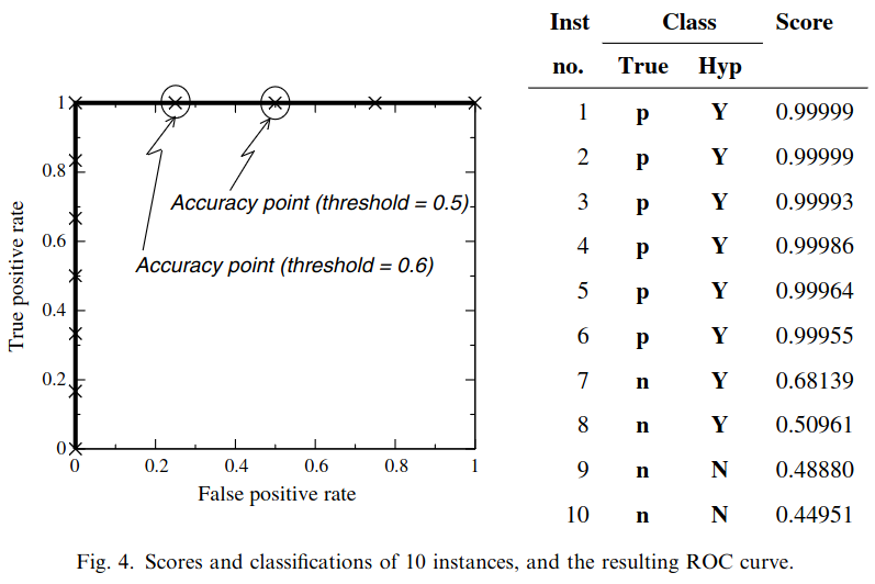{fig-align="center"} ::: footer Fawcett, T. (2006). [*An introduction to ROC analysis*](../refs/Fawcett_2006_Introduction_ROC_Analysis.pdf). Pattern Recognition Letters, 27(8), 861-874. ::: ::: {.notes} Fawcett's Figure 4, and it is the bridge to calibration. Ten instances, scored by a Naive Bayes classifier. The ROC curve is perfect: it goes straight up and then straight across, because every positive outscores every negative. But at the default threshold of 0.5, instances 7 and 8, both negatives with scores 0.68 and 0.51, are called positive, so accuracy is 80 percent. At 0.6 it is 90 percent; anywhere between 0.69 and 0.99 it is 100 percent. Ask them why the two measures disagree. They are measuring different things. The ROC curve measures ranking: does the classifier put positives above negatives? Here it does, perfectly. Accuracy at 0.5 assumes the scores are probabilities, and they are not. Fawcett tries the obvious fix, setting the threshold to the training prior, 6 out of 10 positive, so 0.6, and still gets only 90 percent. Two consequences. First, scores from different kinds of models are not comparable. One model produces scores between 0 and 1, an SVM produces margins that can be any real number, so a common threshold such as 0.5 means nothing across them. Second, there are two remedies. Choose the operating point from the ROC curve itself, or calibrate the scores so that 0.7 really means 70 percent. That second remedy, and why Naive Bayes needs it, is the last third of the lecture. ::: ## Area under an ROC curve (AUC) 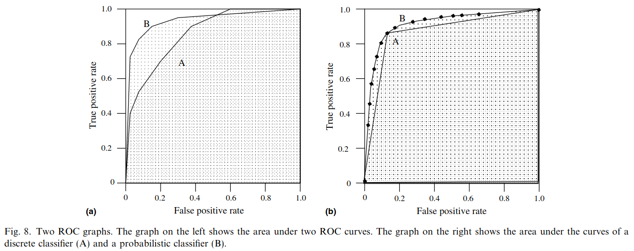{fig-align="center"} ::: footer Fawcett, T. (2006). [*An introduction to ROC analysis*](../refs/Fawcett_2006_Introduction_ROC_Analysis.pdf). Pattern Recognition Letters, 27(8), 861-874. ::: ::: {.notes} AUC, Fawcett's Figure 8. It has a clean interpretation: the probability that a randomly chosen positive is scored above a randomly chosen negative. One is perfect, 0.5 is chance, and below 0.5 means the model is ranking backwards, like E two slides ago. Make that interpretation concrete with the model on the next slide. Its AUC is 0.94. Compare every positive in its test set against every negative, about 390,000 pairs, and the positive has the higher score in 93.9 percent of them: the same number. This is the Wilcoxon, or Mann-Whitney, rank statistic, which is why AUC is sometimes called the c-statistic in medicine. In credit scoring the same quantity is reported as the Gini coefficient, 2 times AUC minus 1. Left panel: B has the larger area and is better on average, but past a false positive rate of 0.6, A is on top. A single number hides crossings, so if you operate at a high false positive rate you would pick the 'worse' model. The reverse case is more common: a screening program only ever operates at the far left of the curve, and two models with the same AUC can behave very differently there. scikit-learn's roc_auc_score has a max_fpr argument that computes the area over that region only, the partial AUC. Right panel: a discrete classifier A is a single point, and its area is what you get by joining it to the corners. It is the scoring classifier B used at one fixed threshold. The two agree at that point, and B is better everywhere else. Summary numbers are for ranking models; the curve is for choosing an operating point. ::: ## ROC curve in sklearn ```{python} #| include: false # Setup code - hidden from slides from sklearn import datasets from sklearn.linear_model import LogisticRegression from sklearn.model_selection import train_test_split X,y = datasets.make_classification(5000, 10, random_state=42) X_train, X_test, y_train, y_test = train_test_split(X, y, random_state=42) clf = LogisticRegression(random_state=0) clf.fit(X_train, y_train) ``` ```{python} #| echo: true #| output-location: column import matplotlib.pyplot as plt from sklearn.metrics import RocCurveDisplay RocCurveDisplay.from_estimator(clf, X_test, y_test, plot_chance_level=True) plt.show() ``` ::: {.notes} Same recipe as the confusion matrix: RocCurveDisplay.from_estimator. If you already have scores rather than a fitted model, from_predictions does the same thing. The setup cell is hidden; it is the same synthetic data and logistic regression, and the figure is live output. plot_chance_level draws the diagonal. The legend reports AUC of 0.94. Connect it to the confusion matrix slide, because it is the same model on the same test set. That matrix was 551, 82, 75 and 542. At the default threshold of 0.5 the model finds 542 of 617 positives, TPR 0.88, and raises 82 false alarms among 633 negatives, FPR 0.13. So the confusion matrix from a few slides back is a single point on this curve, at about (0.13, 0.88). Point at it. Now move along the curve. Suppose false alarms are expensive and you can accept at most 1 percent of them. The threshold has to rise to about 0.93, and TPR falls to 43 percent: it is the same model, and it now misses more than half of the positives. If instead you choose the threshold that maximizes TPR minus FPR, called Youden's J, you get 0.48, almost the default. That is only because this synthetic data is balanced, 617 positives against 633 negatives. On skewed data the defaults stop being sensible. Remind them that AUC says nothing about which of these thresholds to use. ::: ## Multiclass ROC curve :::: {.columns} ::: {.column width="65%"} 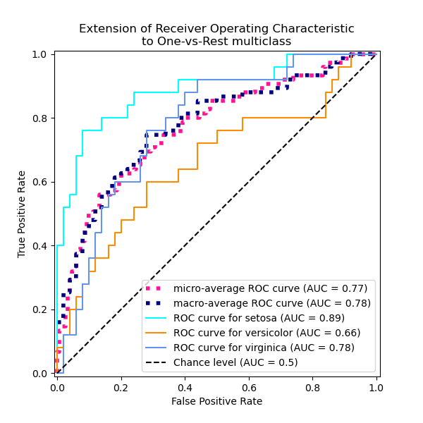{height="760" fig-align="center"} ::: ::: {.column width="35%"} \ **Micro-average:** Pool every one-vs-rest decision into a single curve. Each *sample* counts equally, so the large classes dominate. **Macro-average:** Compute a curve per class, then average them. Each *class* counts equally, so a small, badly served class still shows up. ::: :::: :::footer [code](https://scikit-learn.org/stable/auto_examples/model_selection/plot_roc.html) ::: ::: {.notes} Multiclass ROC from the scikit-learn iris example. ROC is defined for two classes, so we reduce: one-versus-rest gives one curve per class, that class against the other two combined. Setosa 0.89, virginica 0.78, versicolor 0.66, which tells you versicolor is the class the model struggles to separate. If setosa at 0.89 surprises anyone who knows iris, where setosa is trivially separable: the scikit-learn example adds random noise features on purpose, so that the curves are not all perfect. Then two ways to average. Micro pools every one-versus-rest decision across classes and computes one curve, so every sample counts equally and the big classes dominate: 0.77 here. Macro computes each class's curve and averages them, so every class counts equally: 0.78. They are close here because iris is balanced. On imbalanced data they diverge. Tighten the slide's wording here: micro tells you how the model does on a typical sample, and macro is the one that exposes a neglected small class. Which one you report is a decision about whose errors matter. One alternative to mention in passing: one-versus-one, which averages the AUC over every pair of classes (Hand and Till, 2001). It is available as multi_class='ovo' in roc_auc_score, and it is less affected by class imbalance than one-versus-rest. ::: ## ROC Curves: Strengths and Limitations * **What they show:** True Positive Rate (TPR) vs. False Positive Rate (FPR) * **Insensitive to class balance:** by design, since TPR and FPR each stay within one true class. The curve is the same whatever the prevalence * **Limitation:** it never shows precision. At low prevalence a tiny FPR still means most positive predictions are wrong, and the plot gives no warning ::: {.notes} ROC curves are widely used and intuitive, but they have an important limitation. On imbalanced datasets, the false positive rate can appear very small even when the model is making many false positive errors, simply because the denominator (total negatives) is very large. This can make a poor model appear better than it actually is. Put numbers on it, reusing the test from the Wikipedia slide: TPR 90 percent, FPR 5 percent. On the ROC plot that point is close to the top-left corner and looks excellent. Now deploy it where 1 percent of cases are positive. Per 1,000 people: 9 true positives, and 5 percent of 990 negatives, about 50 false positives. Five false alarms for every real case, precision about 15 percent, and nothing on the ROC plot warned you. Fawcett shows the same effect with curves in his Figure 5. He takes two classifiers and multiplies the number of negatives by ten. The ROC curves do not change at all. The precision-recall curves change substantially, and which classifier looks better can flip. A nuance on 'best for balanced datasets'. ROC is not wrong on imbalanced data; its insensitivity to class balance is deliberate, and it is useful when you do not know the prevalence at deployment or it shifts over time. The problem is only that it does not show precision, and on rare-event problems precision is usually what the user feels. Saito and Rehmsmeier (PLOS ONE, 2015) make the case that precision-recall plots are more informative there, which is the next slide. ::: ## Precision-Recall (PR) Curves * **What they show:** Precision (TP / predicted positive) against Recall (TP / actual positive), as the threshold sweeps * **Three cells, not four:** PR uses TP, FP and FN, and ignores the true negatives. It describes the positive class only * **Chance is not the diagonal:** the baseline is a horizontal line at the positive rate, so it drops as positives get rarer * **Summary number:** average precision (AP), the area under the curve * **Advantage:** high precision *and* high recall really is a good model: it finds the positives and most of what it flags is right ::: footer Davis, J., & Goadrich, M. (2006). [*The relationship between Precision-Recall and ROC curves*](https://doi.org/10.1145/1143844.1143874). ICML. Saito, T., & Rehmsmeier, M. (2015). [*The precision-recall plot is more informative than the ROC plot on imbalanced datasets*](https://doi.org/10.1371/journal.pone.0118432). PLOS ONE. ::: ::: {.notes} Precision-Recall curves are often more informative than ROC curves, especially for imbalanced datasets. They focus directly on the performance for the positive class, which is usually the class of interest in imbalanced problems. Start from the previous slide's complaint. Both plots put recall, the true positive rate, on one axis. ROC pairs it with FPR, which is computed inside the negative class; PR pairs it with precision, which is computed inside the predicted-positive column. So PR uses three of the four cells and never touches the true negatives. That is the whole difference, and it is why the plot changes when prevalence changes: precision equals prevalence times TPR, divided by that plus one minus prevalence times FPR. Write that on the board if they want it. Carry the screening example across. That test had TPR 90 percent and FPR 5 percent, a point near the top-left corner of the ROC plot. At 1 percent prevalence it lands at recall 0.9, precision 0.15 in PR space, close to the bottom of the plot. Same classifier, same test set, and now the plot tells you what the user feels. Read the baseline carefully. In ROC space, chance is always the diagonal. In PR space, chance is a horizontal line at the positive rate: 0.5 on balanced data, 0.01 on a 1-in-100 problem. So a PR curve cannot be judged without knowing the prevalence, and two PR plots from different datasets are not comparable. Always say what the baseline is. Three warnings for when they use it. First, the curve is not monotone. One extra false positive among the top-scored instances drops precision sharply, so PR curves are jagged, especially at the left end where precision is computed from a handful of predictions. Second, do not interpolate linearly between points, and do not call trapezoidal area 'the' number. Davis and Goadrich showed that linear interpolation in PR space is misleading; use average precision, which sums precision weighted by the change in recall, which is what scikit-learn's average_precision_score does. Third, their theorem: one curve dominates in ROC space if and only if it dominates in PR space, so the two plots never contradict each other about dominance. What differs is the summary number, and a model tuned to maximize AUC is not necessarily the one with the best average precision. Numbers for the live example on the next slide: prevalence is 0.494, so the chance line is at about 0.49 and the model's AP is 0.94. Read the trade-off off the curve: at 80 percent recall its precision is 90 percent, but pushing recall to 95 percent drops precision to 79 percent. Chasing the last positives always costs precision, and the curve prices it. A correction on attribution, if they have read ahead: the Alsallakh paper does not make the ROC versus PR argument. It uses a recall-precision graph inside its feature view, which you will see later today. The argument is Davis and Goadrich, ICML 2006, and Saito and Rehmsmeier, PLOS ONE 2015, both in the footer. ::: ## Precision-Recall curve in sklearn ```{python} #| include: false # Setup code - hidden from slides from sklearn import datasets from sklearn.linear_model import LogisticRegression from sklearn.model_selection import train_test_split X,y = datasets.make_classification(5000, 10, random_state=42) X_train, X_test, y_train, y_test = train_test_split(X, y, random_state=42) clf = LogisticRegression(random_state=0) clf.fit(X_train, y_train) ``` ```{python} #| echo: true #| output-location: column import matplotlib.pyplot as plt from sklearn.metrics import PrecisionRecallDisplay PrecisionRecallDisplay.from_estimator(clf, X_test, y_test) plt.show() ``` ::: {.notes} And here is how you can generate a Precision-Recall curve in scikit-learn. The `PrecisionRecallDisplay` works similarly to the other display objects we've seen. It takes a classifier and test data to generate the curve. ::: # Visual Analytics Systems for Model Performance ## Squares (2016) 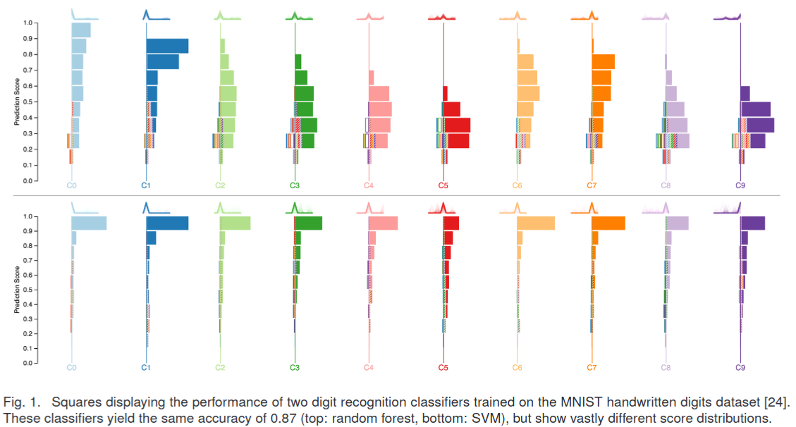{fig-align="center"} :::footer Ren, D., Amershi, S., Lee, B., Suh, J., & Williams, J. D. (2016). [*Squares: Supporting interactive performance analysis for multiclass classifiers*](../refs/Ren_Amershi_Lee_Suh_Williams_2016_Squares_Interactive_Performance_Analysis.pdf). IEEE TVCG. ::: ::: {.notes} Squares, from Microsoft Research, and the reading for today. Read the caption with them because it is the whole argument: two MNIST classifiers, a random forest on top and an SVM below, with the same accuracy, 0.87. One column per class. Within a column, boxes are stacked by prediction score, high at the top. Solid boxes are correct predictions, striped boxes are errors, coloured by the class they were confused with. The SVM is confident: its mass sits at 0.9 and above. The random forest spreads its scores between 0.2 and 0.6. Same accuracy, completely different behaviour, and a confusion matrix would show them as nearly identical. This answers the 'it throws away the scores' complaint from earlier. How the design was decided. They surveyed 102 machine learning practitioners and asked, among other things, how many classes their problems have. Half had built binary classifiers, 41 percent worked with 3 to 20 classes, and only 14 percent went above 20. So they deliberately optimized Squares for 3 to 20 classes, which is what lets them use one distinguishable colour per class. Worth saying out loud in a visualization course: the design space was chosen from data about users, not from what scales best in principle. Three design goals. Show performance at several levels of detail at once, overall, per class and per instance, so a practitioner can decide what to fix first. Be agnostic to the metric, because different problems care about different errors. And keep the instances reachable, so you can click an error and see the actual image. The encoding, in detail. Every box is one instance. Its vertical position is the prediction score. Boxes to the right of a class's axis line are the instances predicted as that class: solid means correct, striped means it was really something else, and the stripe colour names the true class. Boxes to the left are that class's false negatives, outlined rather than filled, coloured by where they went. So each error is drawn twice, once as a false positive in one column and once as a false negative in another, and the colours let you pair them up. That is the trick that makes both error types visible at the same time, which a confusion matrix row-or-column reading does not give you. You can also read the metrics by eye: precision for a class is solid boxes over solid plus striped in its column; recall is solid over solid plus outlined. For big datasets the boxes collapse into stacks, and you expand a class to see individuals. They ran a controlled study: 24 practitioners from an internal mailing list, tasks on 5-class and 15-class problems, Squares against an interactive confusion matrix. Squares was faster, 8.8 seconds against 12.6, and more accurate, 98.9 percent correct against 91.4. The gap was widest on the task 'find an error with a score of 0.9 or above in the wrong class', 7.5 seconds with Squares against 17.4 with the matrix, which is exactly the task a matrix cannot support because it has thrown the scores away. The advantage also grew with the number of classes. ::: --- ::: {.notes} This video demonstrates the Squares system in action. Pay attention to how the interactive nature of the tool allows for a more in-depth analysis of the classifier's performance compared to a static confusion matrix. Three things to point out while it plays. Watch the boxes expand from stacks into individual instances when a class is opened: that is the 'keep the data reachable' goal. Watch hovering over a box show the instance itself and its scores. And watch the striped and outlined boxes pair up by colour as the error is followed from the column that produced it to the class it was taken from. If the video does not load, everything in it is on the previous slide's figure. Remember this deck has to be served over HTTP for YouTube to play. ::: ## Alsallakh et al. (2014) 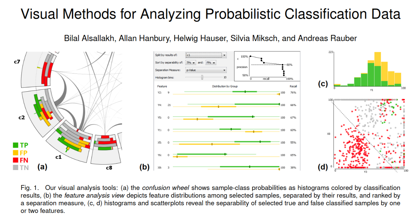{fig-align="center"} :::footer Alsallakh, B., Hanbury, A., Hauser, H., Miksch, S., & Rauber, A. (2014). [*Visual methods for analyzing probabilistic classification data*](../refs/Alsallakh_Hanbury_Hauser_Miksch_Rauber_2014_Visual_Methods_Analyzing_Probabilistic_Classification.pdf). IEEE TVCG. ::: ::: {.notes} Alsallakh and colleagues, TVCG 2014, the teaser. Three linked views. (a) The confusion wheel: one sector per class, histograms of predicted probability inside each sector, coloured green for true positives, yellow false positives, red false negatives, grey true negatives; chords between sectors show confusion. (b) The feature analysis view: for a selected class, which features separate the true positives from the false positives, ranked by a separation measure. (c) and (d) histograms and scatterplots of the chosen features. What makes this paper worth a slide is the task list it starts from. They write down six analysis tasks, and each one involves the predicted probabilities rather than just the counts. Which samples are the model unsure about? How do the true positives, false positives and false negatives differ in their score distributions within a class? Which false negatives have high probability, meaning they are nearly right and cheapest to fix? Which samples are confused between this pair of classes? And, the one the confusion matrix cannot touch at all: can the false positives in a given score range be separated from the true positives by some feature of the data? Their argument is that a matrix gives visual primacy to the confusions, so they build views that give visual primacy to the probabilities and to the features instead. Two design details worth naming. The sectors are ordered so that the thickest chords are the shortest, which reduces crossings, the same kind of layout decision you will make in your projects. And a chord can be split so that the two directions of a confusion are shown separately, because confusion is usually asymmetric. They are honest about the cost, and you should repeat it: a matrix is more accurate for reading off which classes are confused and by how much, because reading a thickness is harder than reading a number. The chord is better for seeing mutual confusion between a pair at a glance. That is a real trade-off, not a win. The idea that carries forward: do not stop at 'which classes are confused', go on to 'which features explain the confusion'. In their own use case, acting on what these views revealed improved the classifier by about 3.5 percent. ::: ## Alsallakh et al. (2014) 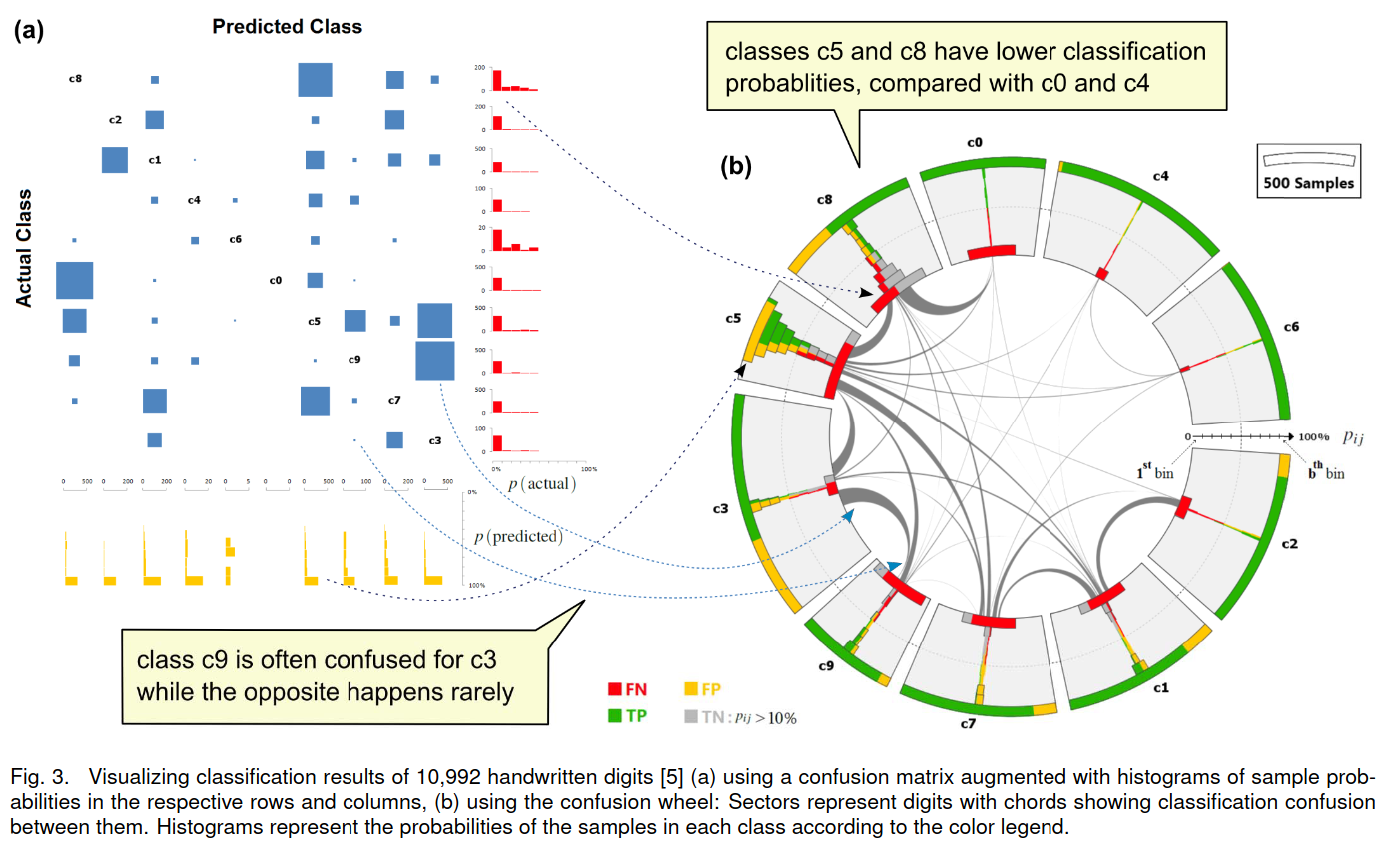{fig-align="center"} :::footer Alsallakh, B., Hanbury, A., Hauser, H., Miksch, S., & Rauber, A. (2014). [*Visual methods for analyzing probabilistic classification data*](../refs/Alsallakh_Hanbury_Hauser_Miksch_Rauber_2014_Visual_Methods_Analyzing_Probabilistic_Classification.pdf). IEEE TVCG. ::: ::: {.notes} The same paper on 10,992 handwritten digits. This is the UCI pen-based dataset, not MNIST: each digit was written on a tablet and is described by 16 numbers, the x and y coordinates of eight points sampled along the pen stroke. That matters for the feature view, because those 16 features are interpretable, which is what makes 'which feature separates these errors' a sensible question. Left, a confusion matrix drawn with squares sized by count and augmented with probability histograms along the rows and columns. Right, the confusion wheel. Read the two callouts: 'class c9 is often confused for c3 while the opposite happens rarely', which is an asymmetry you can see in the chord thickness at each end; and 'c5 and c8 have lower classification probabilities than c0 and c4', which you read off the histograms inside the sectors. Ask them what a plain confusion matrix gives you here. The first callout, with effort, by comparing two cells across the diagonal. The second not at all, because it is a statement about the score distribution, and counts have no scores in them. Then connect it back to our own errors-only matrix earlier: we added the margins, they added whole histograms in each row and column. Same move, more of it. Two more things to note in the left figure. Encoding count as the area of a square is the sort of choice we discussed in the perception lecture; area is judged less accurately than position or length, but it works here because the reader only needs to spot the heavy cells. And the histograms let you distinguish a class the model gets wrong confidently from one it gets wrong while hesitating, which are different problems with different fixes. ::: ## Beauxis-Aussalet and Hardman (2014) 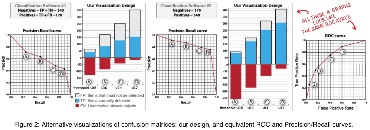{fig-align="center"} :::footer Beauxis-Aussalet, E., & Hardman, L. (2014). [*Visualization of confusion matrix for non-expert users*](../refs/Beauxis_Aussalet_Hardman_2014_Visualization_Confusion_Matrix_Non_Expert_Users.pdf). IEEE VAST. ::: ::: {.notes} Beauxis-Aussalet and Hardman, VAST 2014, designing for non-experts, and the red handwriting is the point. Two classifiers, one tested on 340 negatives and 170 positives, the other with the proportions reversed. Their ROC curves are identical, because ROC is built from within-class rates. Their precision-recall curves differ. And the authors' own design, stacked bars by threshold with true positives in blue, false positives in grey above, and missed objects in red below the axis, shows raw counts, so the difference is obvious. This is the concrete version of 'ROC can mislead under class imbalance': it does not mislead, it simply does not show class proportions, and the end user usually cares about counts. Note where this paper comes from, because it is unusual. The authors work on video-based monitoring of fish populations, and their users are marine ecologists, people who must publish a number for how many fish of a species were in the footage and defend it. Their argument is that the derived metrics we have spent the whole lecture on, precision, recall, F1, are not neutral: each one hides a different error, and a non-expert who picks the wrong one gets a confidently wrong answer. They make the point with two domains that pull in opposite directions: in medical diagnosis a false negative is the expensive error, while in sorting manufactured goods for defects the false positives are what costs you. Be honest about the status of the work: this is a design paper. There is no user study; the authors say the empirical evaluation is future work. So treat the claims as arguments, not evidence. That is a fair thing for your class to notice about a design contribution, and a good question to bring to your own projects: what would you have to run to know this design actually helps? ::: ## Beauxis-Aussalet and Hardman (2014) 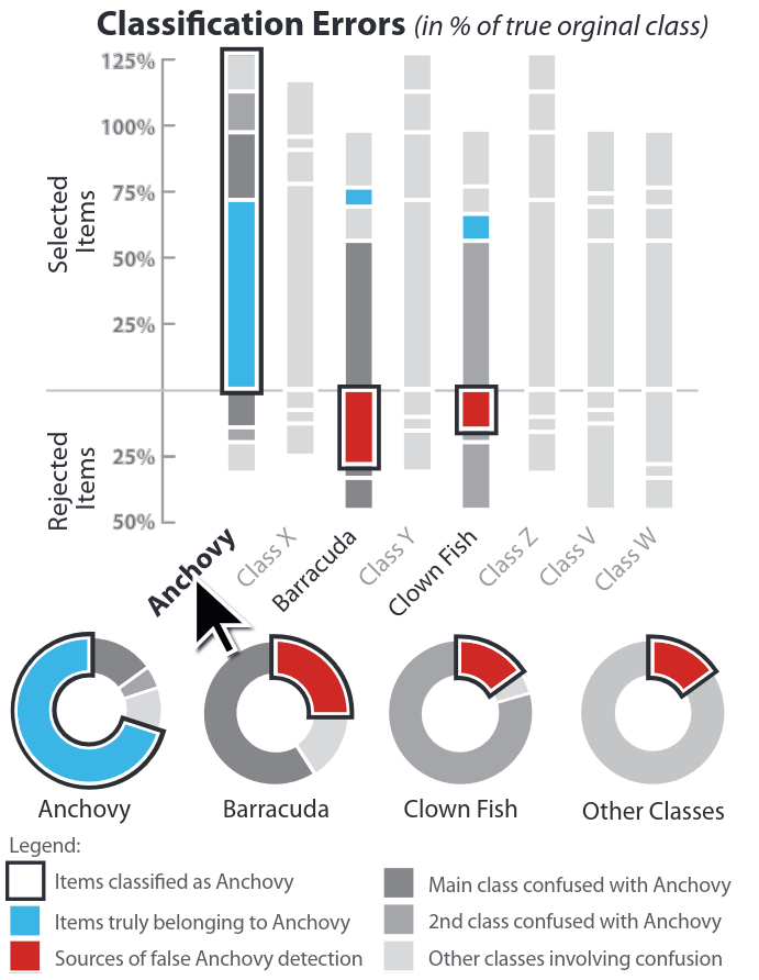{.nostretch width="35%" fig-align="center"} :::footer Beauxis-Aussalet, E., & Hardman, L. (2014). [*Visualization of confusion matrix for non-expert users*](../refs/Beauxis_Aussalet_Hardman_2014_Visualization_Confusion_Matrix_Non_Expert_Users.pdf). IEEE VAST. ::: ::: {.notes} Their design for a multiclass problem, fish species from underwater video, with 'Anchovy' selected. Above the axis: everything classified as anchovy, the blue part truly anchovy, the grey parts other species. Below the axis: true anchovies that were rejected. The red segments in the other columns are where the false anchovy detections came from, here mostly barracuda and clown fish, and the donuts repeat that per class. Percentages are of the true class, which is why a bar can exceed 100 percent. Walk the reading path with them, because the design is doing something specific. The user's question is not 'what is the recall of the anchovy class'. It is 'I am about to report 500 anchovies; how wrong is that number, and which species did it borrow from?'. The design answers it in the order the question is asked: here is what you counted, here is the part that is really anchovy, here is what got mixed in, here is what you missed. Precision and recall are both present, but as parts of a bar rather than as numbers to look up. The design lesson, and it generalizes past this paper: non-experts ask 'of the things you told me were anchovies, how many were?', so answer that question directly rather than handing them a matrix. Worth connecting to the first ten minutes of the lecture: this is the same information as a confusion matrix row and column, re-laid out for someone who will act on the count. ::: ## EnsembleMatrix (2009) 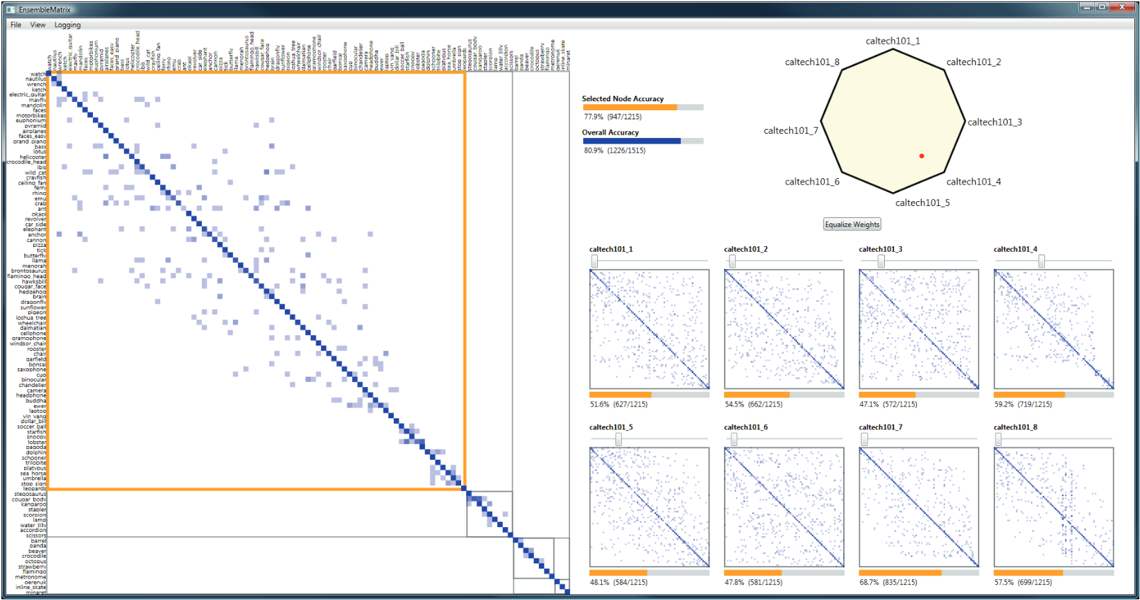{fig-align="center"} :::footer Talbot, J., Lee, B., Kapoor, A., & Tan, D. S. (2009). [*EnsembleMatrix: interactive visualization to support machine learning with multiple classifiers*](../refs/Talbot_Lee_Kapoor_Tan_2009_EnsembleMatrix_Interactive_Visualization_Multiple_Classifiers.pdf). CHI. ::: ::: {.notes} EnsembleMatrix, Talbot and colleagues, CHI 2009, the oldest system today. Caltech-101, eight classifiers trained on different features; their individual confusion matrices are the eight thumbnails, with accuracies from 47 to 69 percent. The polygon at top right is the control: drag the red dot toward a vertex to give that classifier more weight in a linear combination, and the large matrix on the left updates live. Overall accuracy of the combination in this screenshot is 80.9 percent, better than any single member. The orange outline is a partition: you can split the matrix and weight the classifiers differently for different groups of classes. Two design ideas to name. First, the visualization is the control surface: you do not leave it to type parameters, you drag inside the picture of the errors and the picture updates. That is direct manipulation applied to model building, in 2009, well before it was common. Second, partitioning encodes a real insight: different classifiers are good at different parts of the class space, so rather than one global weighting you cut the space and weight separately in each part. The system also keeps the partition honest, since an instance sent to the wrong side can never be recovered, and it draws that fact rather than hiding it. Their study is small but the result is striking. Seven participants, machine learning researchers and non-experts, and they report results for five. In a 30 to 45 minute session those five reached 87.8 percent accuracy on average, from 86.5 to 89. The single classifiers average about 65 percent, and the best hand-built ensemble published at the time was 87.82 percent. So people matched the state of the art in under an hour by dragging in a visualization. Before the task, participants had been asked how long their usual approach would take: answers ran from about a day to more than two weeks. Close the section by lining the four systems up against the three complaints from the confusion matrix slide. Neo takes on scale through hierarchy. Squares and the confusion wheel put the scores back and reach the instances. Beauxis-Aussalet takes on the audience: the reader who is not a machine learning expert. EnsembleMatrix goes furthest, turning the error display into the thing you act on. That is the arc of this section, and the one to remember for your projects: a performance visualization is worth more when it is the place you make the fix. ::: # Calibration ## What is calibration? * When performing classification, we often are interested not only in predicting the class label, but also in the probability of the output * This probability gives us a kind of confidence score on the prediction * However, a model can separate the classes well (having a good accuracy/AUC), but be poorly **calibrated**. In this case, the estimated class probabilities are far from the true class probabilities * We can calibrate the model, changing the scale of the predicted probabilities ::: {.notes} Now we are moving to the third part of our lecture: calibration. Calibration is about whether the probabilities predicted by a model are reliable. For example, if a model predicts a 70% probability of rain, it should rain 70% of the time. A model can be very accurate in its predictions, but still be poorly calibrated. State the definition carefully, because the whole section depends on it. Take every case where the model said 0.7. Among those cases, the positive outcome should happen about 70 percent of the time. That is a statement about a group, not about one prediction: you cannot check calibration on a single case, only on a collection of cases that got the same score. This is why every tool in this section starts by grouping predictions. Then say why anyone should care, because 'the model is 90 percent accurate' usually ends the conversation in practice. Three reasons. First, whenever a human acts on the number: a doctor deciding whether a 30 percent chance of malignancy justifies a biopsy needs 30 percent to mean 30 percent. Second, whenever the score is combined with a cost. The expected-cost calculation multiplies a probability by a money amount, so if the probability is inflated, so is every decision that follows. Third, whenever the score feeds another system, such as a ranking, a threshold rule, or another model downstream. Connect it back to the ROC section. Remember Fawcett's Naive Bayes example: perfect ranking, perfect ROC curve, and scores that were nonsense as probabilities. AUC is invariant to any monotone transformation of the scores, so AUC cannot see miscalibration at all. You can take a perfectly calibrated model, square all its probabilities, and the ROC curve will not move by one pixel. That is the gap this section fills. Last point on the slide's final bullet: calibration is applied after training, as a monotone remapping of the scores, so it never changes the ranking, never changes the ROC curve, and never changes accuracy at a rank-based threshold. It only changes what the numbers mean. ::: ## Calibration - Forecast Example Weather forecasters started thinking about calibration a long time ago (Brier, 1950): a forecast of "70% chance of rain" should be followed by rain 70% of the time. Let's consider a small toy example: :::: {.columns} ::: {.column width="30%"} 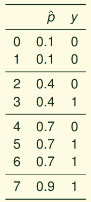{height="600" fig-align="center"} ::: ::: {.column width="70%"} This forecast is doing well at predicting the rain: - "10% chance of rain" was a slight over-estimate: $(\bar{y} = 0/2 = 0\%)$ - "40% chance of rain" was a slight under-estimate: $(\bar{y} = 1/2 = 50\%)$ - "70% chance of rain" was a slight over-estimate: $(\bar{y} = 2/3 = 67\%)$ - "90% chance of rain" was a slight under-estimate: $(\bar{y} = 1/1 = 100\%)$ ::: :::: ::: footer Slides based on [classifier-calibration.github.io](https://classifier-calibration.github.io/) ::: ::: {.notes} The classic motivating example, from the classifier-calibration tutorial this section follows. Eight days, four distinct forecasts. Group the days by forecast and check the outcome: of the two 10 percent days, none had rain; of the two 40 percent days, one did; of the three 70 percent days, two did; the single 90 percent day had rain. Each group is off by a little, in alternating directions. This forecaster is reasonably calibrated. Note what we just did: we binned by predicted value and compared the bin's mean prediction with the bin's observed frequency. That is a reliability diagram, next slide. ::: ## Visualizing forecasts - The Reliability Diagram :::: {.columns} ::: {.column width="30%"} {height="600" fig-align="center"} ::: ::: {.column width="70%"} 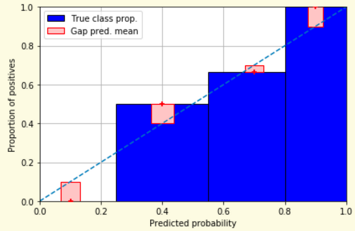{width="100%" fig-align="center"} ::: :::: ::: footer Slides based on [classifier-calibration.github.io](https://classifier-calibration.github.io/) ::: ::: {.notes} The same eight forecasts as a reliability diagram. X is predicted probability, y is the observed proportion of positives. One blue bar per group, its height the observed frequency. The red box is the gap between the bar and the mean prediction in that bin, marked with the plus; the dashed diagonal is perfect calibration. Read it against the table: the 0.1 bin has height zero and a gap of 0.1; the 0.4 bin is at 0.5, the 0.7 bin at 0.67, the 0.9 bin at 1.0. Bars below the diagonal mean over-estimates, above mean under-estimates. ::: ## Reliability diagram - Changing values :::: {.columns} ::: {.column width="30%"} 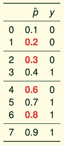{height="600" fig-align="center"} ::: ::: {.column width="70%"} 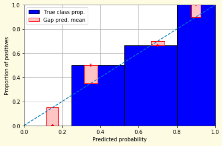{width="100%" fig-align="center"} ::: :::: ::: footer Slides based on [classifier-calibration.github.io](https://classifier-calibration.github.io/) ::: ::: {.notes} Now perturb four of the forecasts, the red values: 0.2, 0.3, 0.6, 0.8. The outcomes have not changed and we keep the same four groups, so the blue bars are identical. What moves is the mean prediction in each bin, to 0.15, 0.35, 0.7 and 0.9, and so the red gaps change. The point: in real data predictions are not repeated values, so we have to bin, and the bin's mean prediction is what gets compared with its observed frequency. ::: ## Reliability diagram - Changing grouping :::: {.columns} ::: {.column width="30%"} {height="600" fig-align="center"} ::: ::: {.column width="70%"} 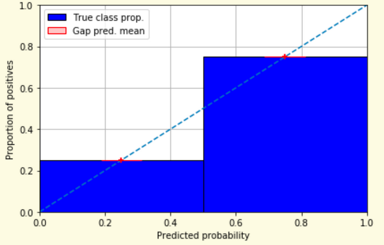{width="100%" fig-align="center"} ::: :::: ::: footer Slides based on [classifier-calibration.github.io](https://classifier-calibration.github.io/) ::: ::: {.notes} Same perturbed forecasts, regrouped into two bins instead of four. Left bin: mean prediction 0.25, one positive in four, observed 0.25. Right bin: mean 0.75, three in four, observed 0.75. Both plus signs sit exactly on the diagonal and the gaps vanish. The model now looks perfectly calibrated. Nothing about the forecasts changed, only the binning. Ask the room which of the last two slides is the truth. Neither: the reliability diagram is an estimate with a hyperparameter, and the second half of this section, Calibrate and Smooth ECE, is about that problem. ::: ## Reliability Diagram in sklearn ```{python} #| include: false from sklearn import datasets from sklearn.linear_model import LogisticRegression from sklearn.naive_bayes import GaussianNB from sklearn.model_selection import train_test_split X,y = datasets.make_classification(5000, 10, random_state=42) X_train, X_test, y_train, y_test = train_test_split(X, y, random_state=42) lg = LogisticRegression(random_state=0) nb = GaussianNB() lg.fit(X_train, y_train) nb.fit(X_train, y_train) ``` ```{python} #| echo: true #| output-location: column import matplotlib.pyplot as plt from sklearn.calibration import CalibrationDisplay fig = plt.figure() ax = fig.add_subplot(111) CalibrationDisplay.from_estimator(lg, X_test, y_test, n_bins=10, ax=ax, label='Logistic Regression') CalibrationDisplay.from_estimator(nb, X_test, y_test, n_bins=10, ax=ax, label='Naive Bayes') ``` ::: {.notes} Two classifiers on the same synthetic data: logistic regression and Gaussian Naive Bayes, set up in a hidden cell. CalibrationDisplay.from_estimator with ten bins, both on one axis; the figure on the right is live output. Logistic regression hugs the diagonal, which is expected because it is trained by minimizing log-loss, a proper scoring rule. Naive Bayes bends away from it: its independence assumption counts correlated evidence several times and pushes probabilities toward 0 and 1. Both have similar accuracy. Next slide names the shapes. ::: ## Common sources of miscalibration * **Underconfidence:** a classifier thinks it's worse at separating classes than it actually is. - Underconfidence typically gives sigmoidal distortions - To calibrate these means to pull predicted probabilities away from the centre * **Overconfidence:** a classifier thinks it's better at separating classes than it actually is - Here, distortions are inverse-sigmoidal - Calibrating these means to push predicted probabilities toward the centre A classifier can be overconfident for one class and underconfident for the other ::: {.notes} Miscalibration can occur in two main ways: underconfidence and overconfidence. Underconfident models produce probabilities that are too close to 0.5, while overconfident models produce probabilities that are too close to 0 or 1. The shape of the reliability diagram can help us diagnose which of these problems is occurring. Get the shapes straight, because the slide's wording is terse and the words are easy to swap. Take an overconfident model. It says 0.95 when the truth is 0.75, and 0.05 when the truth is 0.25. Plot predicted against observed: at the high end the curve falls below the diagonal, at the low end it rises above. The curve is flatter than the diagonal through the middle and steep at the ends. That is the inverse-sigmoid shape. An underconfident model is the mirror image: it says 0.6 when the truth is 0.9, so the curve is above the diagonal at the high end and below at the low end, steeper than the diagonal in the middle. That is the sigmoid shape. Two rules of thumb they can use on any reliability diagram. Below the diagonal means the model promised more than it delivered, so it is overconfident there. And the direction of the fix follows the shape: to fix overconfidence, pull the probabilities toward the centre; to fix underconfidence, push them away from it. Where each one comes from is worth a sentence. Overconfidence comes from models that keep driving the training loss down after they have stopped getting more accurate, which is exactly Guo's story about deep networks, two slides ahead. It also comes from Naive Bayes, which multiplies evidence that is not independent and so counts the same information several times. Underconfidence is typical of methods that hedge: max-margin methods such as SVMs, which were never trained to output probabilities at all, and averaging methods such as random forests, where a prediction near 1 requires every tree to agree. And take the last line on the slide seriously: overconfident for one class and underconfident for the other is common in imbalanced problems, which is one reason a single ECE number is not enough. ::: ::: footer Slides based on [classifier-calibration.github.io](https://classifier-calibration.github.io/) ::: ## Reliability Diagram in sklearn 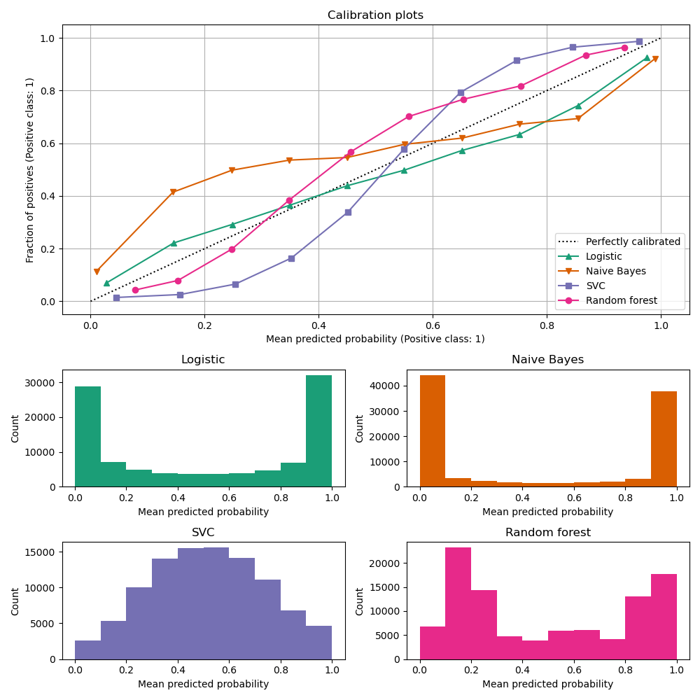{.nostretch width="45%" fig-align="center"} :::footer [code](https://scikit-learn.org/stable/modules/calibration.html) ::: ::: {.notes} The scikit-learn comparison, four models, and it puts a face on both failure modes from the previous slide. Naive Bayes, orange: an inverse-sigmoid, above the diagonal at low predictions and below it at high ones. It says 0.15 when the truth is 0.4 and 0.85 when the truth is 0.7, and its histogram below is piled at 0 and 1. That is overconfidence. The SVC, purple: a sigmoid, and its histogram is a hump in the middle; it rarely commits. That is underconfidence, typical of max-margin methods. Random forest, pink, is mildly sigmoid too, because averaging trees pulls predictions away from 0 and 1. Logistic regression, green, is close to the diagonal. Always read the histogram with the curve: it tells you where the curve is supported by data. ::: ## Calibration metrics Let $N$ be the total number of samples, $B$ the number of bins, $n^b$ the samples in bin $b$, $acc(b)$ the fraction of positives in bin $b$, and $conf(b)$ the average predicted probability in bin $b$. - Expected Calibration Error: $ECE = \sum_{b=1}^B \frac{n^b}{N}|acc(b) - conf(b)|$ - Maximum Calibration Error: $MCE = \underset{b \in \{1,2,\dots,B\}}{\text{max}} |acc(b) - conf(b)|$ ::: {.notes} Besides visualizing calibration with reliability diagrams, we can also quantify it using metrics like Expected Calibration Error (ECE) and Maximum Calibration Error (MCE). ECE gives an overall measure of miscalibration, while MCE tells us the worst-case deviation. Read the ECE formula as a weighted average, because that is all it is. In each bin, take the gap between what the model promised, conf(b), and what happened, acc(b). Weight each gap by the share of the samples in that bin, and add them up. So ECE is the average vertical gap in the reliability diagram, with bins that hold more samples counting more. MCE takes the largest gap instead of the average, which is what you want when a single bad region is unacceptable, for example a medical cutoff. Both are in the same units as probability, so an ECE of 0.05 means the model is off by 5 percentage points on average. Two warnings. First, the notation: this slide writes acc(b) as the fraction of positives in the bin, which is the binary, positive-class version. Guo's paper, coming up, uses a different convention: bin by the confidence of the predicted class, whatever that class is, and compare against the accuracy in the bin. Both are called ECE and they do not give the same number on a multiclass problem. Whenever they read an ECE in a paper, they should find out which one it is. Second, and this is the thread that runs to the end of the lecture: ECE is not a property of the model. It is a property of the model plus a binning choice, the number of bins and whether they are equal-width or equal-count. Change that choice and the number changes. We saw a two-bin example turn a visibly miscalibrated model into a perfect one earlier. The Calibrate slide shows it at full scale, and Smooth ECE is an attempt to remove the choice altogether. Also worth saying: ECE has no penalty for being useless, which is the next slide. ::: ## Perfectly Calibrated, and Useless * Predict the base rate for everyone: *"there is a 5% chance you have the disease"*, for every patient alike * Every group's observed frequency matches its prediction, so **ECE = 0** and the reliability diagram sits on the diagonal * Yet it ranks nobody above anybody: **AUC = 0.5**, and it never identifies a single patient * **Calibration** is being right *on average*; **sharpness** is *committing* to a prediction. A useful model needs both * Recalibration can repair a sharp but miscalibrated model. Nothing repairs an unsharp one ::: {.notes} SKIPPABLE - if running long, jump to Calibration of modern models. The counterexample that keeps calibration honest, and it costs two minutes. Go back to the disease model from the first ten minutes of the lecture, but instead of predicting the label, have it output 0.05 for everybody, the prevalence. Check it against the definition. Group the cases by predicted value: there is one group, everyone, with prediction 0.05, and 5 percent of them are positive. The prediction matches the observed frequency exactly, so the gap is zero in every bin and ECE is zero. On a reliability diagram it is a single point sitting on the diagonal. By the definition we have been using all section, this model is perfectly calibrated, and it is worth pausing so the room feels how wrong that sounds. Now measure the other thing. Every case gets the same score, so no positive is ranked above any negative: AUC is 0.5, chance. It never picks out a patient. In the decomposition from the proper scoring rules slides, its calibration loss is zero and its refinement loss is as large as it can be, and refinement loss is the part that no recalibration can fix. So the pairing to remember is calibration and sharpness. Sharpness is how far the predictions get away from the base rate, how willing the model is to commit. Calibration asks whether those commitments are honest. A weather forecaster who says 30 percent every day, the climatological average, is perfectly calibrated and useless; the good forecaster says 5 percent and 95 percent on the right days and is still right on average. The practical rule for their projects: never report ECE on its own. Report it next to AUC, or report a proper scoring rule, which charges for both failures at once. Brier score for the constant model here is 0.05 times 0.95, about 0.0475, and any model that actually discriminates will beat that. ::: ## Calibration of modern models 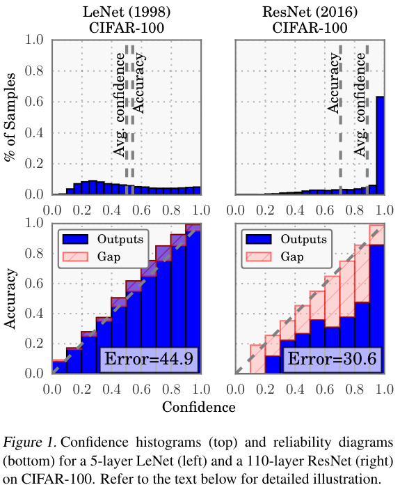{.nostretch width="35%" fig-align="center"} :::footer Guo, C., Pleiss, G., Sun, Y., & Weinberger, K. Q. (2017). [*On calibration of modern neural networks*](../refs/Guo_Pleiss_Sun_Weinberger_2017_Calibration_Modern_Neural_Networks.pdf). ICML. ::: ::: {.notes} Figure 1 of Guo et al., ICML 2017, the paper that made calibration a deep learning topic. Two networks on CIFAR-100: a 5-layer LeNet from 1998 and a 110-layer ResNet from 2016. Top row, confidence histograms: LeNet's average confidence roughly equals its accuracy, the two dashed lines coincide; the ResNet's confidence is piled up near 1 and its average confidence is well above its accuracy. Bottom row, reliability diagrams: LeNet's bars follow the diagonal; the ResNet's sit well below it with large red gaps. Careful with the numbers in the boxes: 'Error' is classification error, 44.9 versus 30.6 percent. So the ResNet is much more accurate and much worse calibrated. Their explanation: depth, width, batch norm and less weight decay let the network keep reducing log-loss by becoming more confident after accuracy stops improving. Their fix is temperature scaling, a one-parameter Platt scaling. ::: ## Calibration of modern models :::: {.columns} ::: {.column width="30%"} 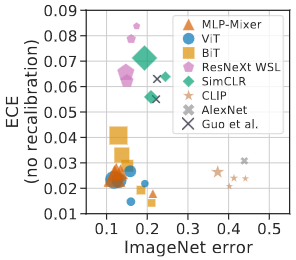{width="100%"} ::: ::: {.column width="70%"} 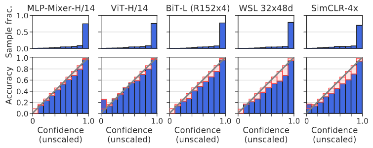{width="100%"} ::: :::: **Architecture and pre-training, not size, drive calibration: ViT and MLP-Mixer are both the most accurate and among the best calibrated. In-distribution, calibration degrades slightly with size; under distribution shift the effect reverses** :::footer Image taken from Minderer, Matthias, et al. (2021). *Revisiting the calibration of modern neural networks*. Advances in Neural Information Processing Systems. ::: ::: {.notes} Minderer et al., NeurIPS 2021, revisiting that story four years on. Left: ECE against ImageNet error for several model families, marker size is model size. Guo's conclusion would predict that the accurate models in the bottom left are badly calibrated. They are not: the vision transformers and MLP-Mixers are both the most accurate and among the best calibrated, while the ResNeXt WSL and SimCLR families sit higher. Right: reliability diagrams for five of them, the gaps small for Mixer, ViT and BiT and visibly larger for WSL and SimCLR. Their reading: architecture and pretraining matter more than size, and the trend 'bigger means worse calibrated' was a property of a generation of convolutional nets, not a law. The general lesson for the class: measure calibration for your model, do not inherit it from a paper. ::: ## Is the 2017 Story Still True? * **The observation held:** those CNNs really were overconfident, and temperature scaling really does fix them cheaply * **The extrapolation did not.** A benchmark over 117,000 architectures finds *no* universal accuracy-calibration trade-off, and attributes "calibration decreases with model size" to **survivorship bias** in the 2017 model grid * **The direction has flipped for foundation models:** ConvNeXt, EVA and BEiT come out *under*confident in-distribution, though better calibrated under distribution shift * **For LLMs:** pre-trained next-token probabilities are close to calibrated; **SFT and RLHF degrade that**. For RLHF'd models, asking for a *stated* confidence often beats the token probabilities * **So:** measure calibration for *your* model on *your* distribution. Do not inherit a trend from a paper ::: footer Tao, L. et al. (2024). [*A Benchmark Study on Calibration*](https://arxiv.org/abs/2308.11838). ICLR. Hekler, A. et al. (2025). [*Beyond Overconfidence*](https://arxiv.org/abs/2506.09593). arXiv preprint. Tian, K. et al. (2023). [*Just Ask for Calibration*](https://aclanthology.org/2023.emnlp-main.330/). EMNLP. ::: ::: {.notes} SKIPPABLE - if running long, jump to Proper Scoring Rules. Where the field actually stands, because Guo's paper is cited constantly and its headline is now quoted past what it supports. Be precise about which part survived. The observation survived. Those networks, on those datasets, were overconfident, and the reliability diagram showed it. Temperature scaling is still the first thing to try, it is one parameter, and it cannot change accuracy. The generalization did not survive. Tao and colleagues, ICLR 2024, evaluated calibration across more than 117,000 architectures from a neural architecture search space, rather than the handful of ResNet variants Guo could afford in 2017. They find that higher accuracy goes with better calibration among the strong models, that the relationship disappears across all architectures, and, in their own words, that the earlier 'calibration decreases with model size' conclusion may be survivorship bias: the models people kept and published were not a random sample. That is a nice methodological point for this class. A trend measured over the models that happened to exist in 2017 was read as a law about neural networks. Then the direction reversed. Hekler and colleagues, 2025, looked at foundation-scale vision models, ConvNeXt, EVA and BEiT, and found them underconfident in-distribution, the opposite failure, while being better calibrated under distribution shift than their predecessors. Flag the status honestly: this is an arXiv preprint, not peer reviewed, so treat it as a signal rather than a settled result. The LLM part is the one they will use. Pre-trained language models have famously well-calibrated next-token probabilities; the GPT-4 report showed that the pre-trained model was close to calibrated on multiple-choice questions and that the post-RLHF model was substantially worse. The intuition is worth stating: the reward model prefers answers that sound decisive, so hedging is trained out. Tian and colleagues, EMNLP 2023, found that for RLHF-tuned models, the confidence the model states in words is often better calibrated than the probability it assigns to the tokens, which is a strange and useful fact. If anyone is doing a project on LLM outputs, this is the paper to start from. The takeaway is the same one the section has been building: calibration is a property of a model on a distribution, measured with a choice of estimator. All three of those can change under you. ::: ## Proper Scoring Rules :::: {.columns} ::: {.column width="40%"} * Proper scoring rules are calculated at the observation level, whereas ECE is binned * Think of them as putting each item in its separate bin, then computing the average of some loss for each predicted probability and its corresponding observed label ::: ::: {.column width="60%"} 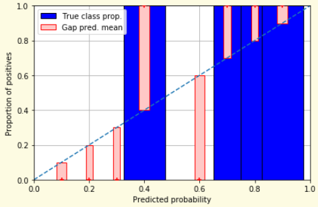{width="100%" fig-align="center"} ::: :::: ::: footer Slides based on [classifier-calibration.github.io](https://classifier-calibration.github.io/) ::: ::: {.notes} Proper scoring rules evaluate each prediction on its own rather than per bin. The figure is the limit of the last three slides: give every distinct prediction its own bin. Each bar is then either 0 or 1, the observed label, and the red gap is the distance from the prediction to that label. Average a loss over those gaps and you have a scoring rule. 'Proper' means the expected score is optimized by reporting your true belief, so a model cannot game it by shading its probabilities. ::: ## What Makes a Scoring Rule *Proper*? * You believe $q$, you report $p$. Your expected score is $\ q\,S(p,1) + (1-q)\,S(p,0)$ * **Proper:** $p = q$ is optimal. **Strictly proper:** $p = q$ is the *only* optimum, so honesty is uniquely best * **Accuracy is not *strictly* proper.** Believing 0.6, claiming $1.0$ scores exactly the same: every report above $0.5$ ties. It cannot tell $0.51$ from $0.99$ * **Absolute error $|p - y|$ is worse:** its expectation $q + p(1 - 2q)$ is *linear* in $p$, so the unique optimum is $p = 0$ or $1$. It pays you to overclaim * A metric that is indifferent to your uncertainty, or rewards overstating it, cannot judge probabilities. Next: two that do neither ::: {.notes} SKIPPABLE - if running long, jump to the Brier and log-loss formulas. The definition behind the word we keep using, and it takes two minutes. Set it up as a bet. You have an honest belief q that the outcome is positive. You are allowed to report any number p, and you will be scored by some rule S. Your expected score, computed under your own belief, is q times the score when it happens plus one minus q times the score when it does not. A rule is proper when that expression is best at p equal to q, and strictly proper when p equal to q is the only best answer. In plain terms: you cannot do better by lying about your uncertainty. Now the two counterexamples, and do them in this order because the first one is the one they use every day. Be careful to separate proper from strictly proper here, because the two counterexamples fail in different ways and the difference is the interesting part. Accuracy. Score a forecast by whether it rounds to the right label. If you believe 0.6, what should you report? Let them answer, then give the exact result: every report above 0.5 gives identical expected accuracy, 0.6 and 0.99 and 1.0 alike. So the honest answer is among the best, which makes accuracy technically proper, but it is not strictly proper, because nothing singles honesty out. Accuracy is simply indifferent to the difference between 0.51 and 0.99. That is the formal version of the complaint we opened the lecture with: it cannot see confidence at all, so it cannot detect miscalibration in either direction. Absolute error. This one usually surprises people, since squared error is proper and absolute error feels similar. Expand the expectation: q times one minus p, plus one minus q times p, equals q plus p times one minus two q. That is linear in p, so it has no interior optimum. If q is above a half you should report 1, if below you should report 0. So this one is actively improper: it does not merely fail to reward honesty, it pays you to overclaim. Absolute error on probabilities is a threshold rule in disguise. Compare with the Brier score on the next slide, where the expectation is quadratic and its derivative is twice p minus q: zero exactly at the honest answer, pushing down if you overstate and up if you understate. That is properness, mechanically. Two remarks if there is time. First, this is why cross-entropy is the training loss: minimizing a strictly proper scoring rule has the true conditional probability as its optimum, which is why logistic regression hugs the diagonal and Naive Bayes, which is not fitted that way, does not. Second, connect back to the slide where the base-rate model had ECE zero: ECE is not a proper scoring rule either, and that is the cleanest way to say why it cannot be your only number. ::: ## Proper Scoring Rules * Brier Score/Quadratic error/Euclidean distance: $$BS = \frac{1}{N} \sum_{i=1}^N (\hat{y}_i - y_i)^2$$ * Log-loss/Cross entropy: - Frequently used as the training loss of machine learning methods, such as neural networks - Only penalises the probability given to the true class $$LL = -\frac{1}{N} \sum_{i=1}^N [y_i \text{log}(\hat{y}_i) + (1-y_i)\text{log}( 1 - \hat{y}_i)]$$ ::: footer Slides based on [classifier-calibration.github.io](https://classifier-calibration.github.io/) ::: ::: {.notes} The two you will meet. Brier score is mean squared error on probabilities: bounded between 0 and 1 in this binary form, easy to interpret. Log-loss is cross-entropy, the training loss of most neural networks and of logistic regression, which is why those models tend to be calibrated on their training distribution. The practical difference is in the tails: log-loss goes to infinity if you assign probability zero to something that happens, Brier is forgiving. Both reward calibration and sharpness together, which is the next slide. ::: ## Proper Scoring Rules An intuitive way to decompose proper scoring rules is into refinement and calibration losses * **Refinement loss:** is the loss due to producing the same probability for instances from different classes * **Calibration loss:** is the loss due to the difference between the probabilities predicted by the model and the proportion of positives among instances with the same output ::: footer Slides based on [classifier-calibration.github.io](https://classifier-calibration.github.io/) ::: ::: {.notes} The decomposition, due to Murphy and generalized by Kull and Flach. Every proper score splits into two parts. Refinement loss: you gave the same probability to instances that differ in class, which is a failure to discriminate, and no recalibration can fix it. Calibration loss: within a group that received the same prediction, the prediction differs from the observed frequency, which a monotone remapping can fix. This is why calibration methods on the next slides never change the ranking, and therefore never change the ROC curve or AUC: they only attack the second term. ::: ## Calibration Techniques **Parametric** calibration involves modelling the score distributions within each class - **Platt scaling:** Logistic calibration can be derived by assuming that the scores within both classes are normally distributed with the same variance (Platt, 2000) - **Beta calibration:** employs Beta distributions instead, to deal with scores already on a [0, 1] scale (Kull et al., 2017) - **Dirichlet calibration** for more than two classes (Kull et al., 2019) **Non-parametric** calibration often ignores scores and employs ranks - **Isotonic regression** fits a non-parametric isotonic regressor, which outputs a step-wise non-decreasing function ::: footer Slides based on [classifier-calibration.github.io](https://classifier-calibration.github.io/) ::: ::: {.notes} The map of methods, all of which learn a function from the model's score to a probability on held-out data. Parametric methods assume a shape. Platt scaling fits a sigmoid and is what you get from assuming Gaussian class-conditional scores with equal variance. Beta calibration handles scores already in [0,1] and can fit inverse-sigmoid shapes that Platt cannot. Dirichlet is the multiclass generalization, and temperature scaling for neural nets is its one-parameter special case. Non-parametric: isotonic regression assumes only monotonicity. Two practical rules: always fit the calibrator on data the model was not trained on, and choose by data size, parametric when you have hundreds of samples, isotonic when you have thousands. ::: ## Platt scaling * Assumes the calibration curve can be corrected by applying a sigmoid to the raw predictions. This means finding $\mathbf{A}$ and $\mathbf{b}$ via MLE: $p(y_i = 1 | \hat{y}_i) = \frac{1}{1 + exp(\mathbf{A}\hat{y}_i + \mathbf{b})}$ * Works best if the calibration error is symmetrical (classifier output for each binary class is normally distributed with the same variance) * This can be a problem for highly imbalanced classification problems, where outputs do not have equal variance * In general it is most effective when the un-calibrated model is under-confident and has similar calibration errors for both high and low outputs ::: {.notes} Platt scaling is a simple and widely used calibration method. It learns a logistic regression model on the outputs of the original model. This method is most effective when the calibration error is symmetric, but it can be less effective for imbalanced datasets. Say what is actually being fit, because the formula on the slide hides it. You take the model's raw scores on held-out data, and you fit a one-dimensional logistic regression from score to label: two parameters, a slope A and an intercept b, fitted by maximum likelihood. The output is a sigmoid that maps scores to probabilities. It came from Platt's work on SVMs, where the raw output is a margin, a number with no probabilistic meaning at all, so something had to convert it. The assumption behind it is the second bullet, and it is worth making concrete: it is what you get if the scores of the positives and the scores of the negatives are both normal with the same variance. If that holds, the sigmoid is exactly right. If the two classes have different spreads, which is common under imbalance, the true curve is not a sigmoid and Platt cannot represent it. Emphasize the practical rule: fit the calibrator on data the model has not seen. If you fit it on the training set, the scores there are already over-separated and the calibration map will be wrong in the direction that matters. In scikit-learn this is CalibratedClassifierCV, with method='sigmoid', which does the held-out fitting with cross-validation for you. Its great virtue is that two parameters almost never overfit, so it is the right choice when the calibration set is small, hundreds of samples rather than thousands. Its limit is shape: it can only bend a sigmoid. Two slides from now you will see it fail on Naive Bayes, whose distortion has the opposite curvature, and succeed on an SVM, whose distortion is a sigmoid. The deep learning version, temperature scaling, is coming up in a moment. ::: ## Isotonic regression * Fits a non-parametric isotonic regressor, which outputs a step-wise non-decreasing function * Isotonic regression is more general when compared to Platt scaling, as the only restriction is that the mapping function is monotonically increasing * Is more powerful as it can correct any monotonic distortion of the un-calibrated model * However, it is more prone to overfitting, especially on small datasets ::: {.notes} Isotonic regression is a more powerful, non-parametric calibration method. It can correct any monotonic distortion in the model's outputs. However, because it is more flexible, it is also more prone to overfitting, especially when the dataset is small. What it does, concretely. Sort the held-out samples by score. Now find the non-decreasing step function that best fits the labels in least squares. The classical algorithm is pool-adjacent-violators: walk along the sorted list, and whenever a later group has a lower average label than the group before it, which violates monotonicity, merge the two and use their pooled average. Repeat until nothing is out of order. The result is a staircase, and the height of each step is the observed fraction of positives among the scores that landed on it. So the only assumption is the ordering: it trusts the model's ranking and rewrites the values. That is also the honest way to say what calibration can and cannot do, which we saw in the refinement-versus-calibration decomposition: if the ranking is wrong, no monotone map will save it. Two practical consequences. First, it needs data. Each step is an average over the samples that fall in it, so with a few hundred calibration samples the staircase is fitted to noise. The usual advice is Platt when you have hundreds, isotonic when you have thousands. Second, it cannot extrapolate: outside the range of scores it saw during fitting, it is flat, and it maps everything to the extreme step. In scikit-learn it is CalibratedClassifierCV with method='isotonic'. Also point out the visual signature, so they can recognize it two slides on: a calibrated isotonic curve is a staircase, not a smooth curve, and its histogram of predictions shows spikes at the step values rather than a continuous spread. ::: ## Temperature Scaling * Guo et al.'s fix for a modern network: divide the logits by a single learned scalar $T$ before the softmax $$\hat{q}_i = \max_k \ \sigma_{SM}(z_i / T)^{(k)}$$ * $T > 1$ *softens* the distribution (raises its entropy); $T = 1$ leaves the network unchanged; $T \to \infty$ gives uniform * $T$ is fitted by minimising NLL on a **held-out validation set**. The network's weights are never touched * Dividing every logit by the same number cannot change which one is largest, so **accuracy is unchanged** * One parameter, so it rarely overfits: the special case of Platt scaling used for deep nets today ::: footer Guo, C., Pleiss, G., Sun, Y., & Weinberger, K. Q. (2017). [*On calibration of modern neural networks*](../refs/Guo_Pleiss_Sun_Weinberger_2017_Calibration_Modern_Neural_Networks.pdf). ICML. ::: ::: {.notes} SKIPPABLE - if running long, jump to Calibration in sklearn. The method Guo's paper recommends, and the one they are most likely to use, because it is what deep learning libraries do. A classifier's last layer produces logits, and the softmax turns them into probabilities. Temperature scaling inserts one division: every logit is divided by the same positive number T before the softmax. Build the intuition on the two limits. With T equal to 1 nothing changes. As T grows, the logits are squeezed together, the softmax output flattens, and in the limit every class gets 1 over K: maximum uncertainty. With T below 1 the opposite, the distribution sharpens. A network that is overconfident is fixed by a T greater than 1, and in practice the fitted value for an overconfident vision model is somewhere above 1. Two properties make it attractive. First, the argmax cannot move, because dividing every logit by the same positive number preserves their order. So accuracy, and the confusion matrix, and the ROC curve, are all exactly what they were. The only thing that changes is the probability attached to the prediction. Second, one parameter cannot overfit a validation set of any reasonable size, which is why it beats the fancier variants such as matrix scaling in Guo's own experiments. The one thing to insist on: T is fitted on held-out data by minimizing negative log-likelihood. Fit it on the training set, where the network is already overconfident by construction, and you will learn T close to 1 and fix nothing. Connect it to the two methods before it: this is Platt scaling with the slope shared across all classes and the intercept dropped, applied to logits rather than to scores. And connect it forward: it is a monotone map, so it changes no ranking, which is the same reason isotonic and Platt leave the ROC curve alone. If anyone asks about LLMs, this is the same temperature as in sampling, applied for a different purpose. ::: ## Calibration in sklearn 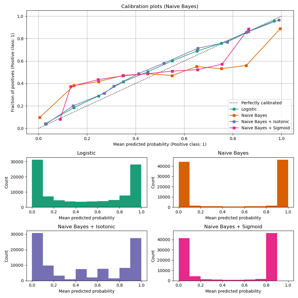{.nostretch width="45%" fig-align="center"} :::footer [code](https://scikit-learn.org/stable/auto_examples/calibration/plot_calibration_curve.html) ::: ::: {.notes} The scikit-learn calibration example, Naive Bayes. The uncalibrated curve, orange, is the inverse-sigmoid of an overconfident model, and its histogram is two spikes at 0 and 1. Isotonic regression, purple, brings it onto the diagonal alongside logistic regression. Platt or sigmoid scaling, pink, barely helps: it still sits well off the diagonal between 0.2 and 0.8. That is the point of the slide. Platt can only fit a sigmoid-shaped distortion, and this one has the opposite shape. Note also what calibration does to the histograms: isotonic spreads the predictions back across the range. ::: ## Calibration in sklearn 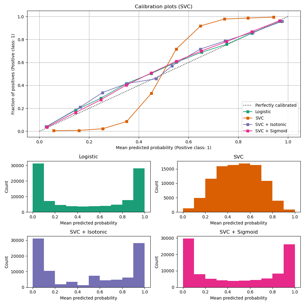{.nostretch width="45%" fig-align="center"} :::footer [code](https://scikit-learn.org/stable/auto_examples/calibration/plot_calibration_curve.html) ::: ::: {.notes} Same example with a linear SVC. Now the uncalibrated curve is a clean sigmoid, the underconfident shape, with its histogram humped in the middle. Here both methods work: sigmoid and isotonic land on the diagonal and are indistinguishable from logistic regression. Put the two slides side by side in their heads: Platt scaling fixes underconfident sigmoid distortions and fails on overconfident ones; isotonic fixes both but needs more data. Diagnose the shape before choosing the method. ::: ## Calibration Takeaways * Reliability diagrams are a standard way to visualize calibration * ECE is a summary of what reliability diagrams show * Proper scoring rules (Log loss, Brier score) measure different aspects of probability correctness * However, proper scoring rules cannot tell us where a model is miscalibrated * **Calibration is not quality:** the base-rate predictor scores ECE 0. Always report it beside AUC or a proper scoring rule * **Every number here depends on the binning**, which papers rarely report. The rest of this section is about that ::: {.notes} To summarize the key points on calibration: reliability diagrams are the primary tool for visualizing calibration. ECE and MCE are metrics to quantify it. Proper scoring rules like Brier score and log-loss provide a more detailed view of the correctness of the predicted probabilities. Add the two warnings on the slide, because they are what the rest of the section is about. First, calibration is not quality. The base-rate predictor is perfectly calibrated and worthless, so always report calibration next to a measure of discrimination such as AUC, or use a proper scoring rule, which charges for both at once. Second, every number on this slide depends on a binning choice that nobody reports. That is the cue for the next four slides: the Calibrate paper shows how much the picture moves when you change bins, our learned reliability diagram avoids the bins by fitting a curve, and Smooth ECE avoids them with kernel smoothing and hands you an error bar. If you want one practical recipe for their projects: hold out a calibration set, plot the reliability diagram with a couple of different bin counts to see whether your conclusion survives, report Brier or log-loss alongside AUC, and if the curve is off, choose the repair by its shape, Platt or temperature for a sigmoid, isotonic when you have enough data. ::: ## Hyperparameters of reliability diagrams 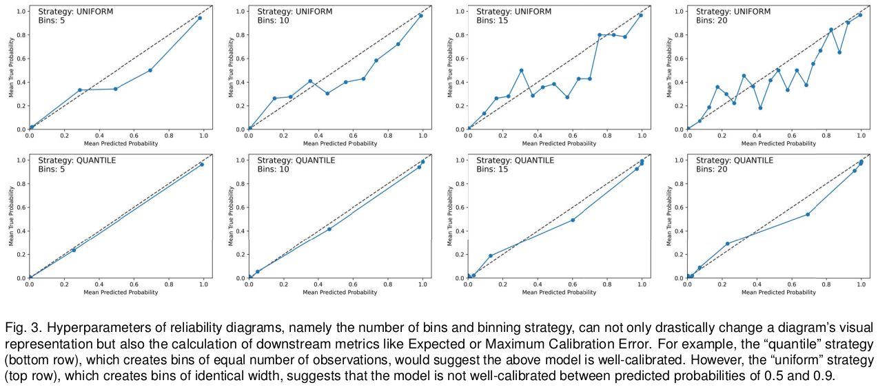{fig-align="center"} :::footer Image taken from Xenopoulos, P., Rulff, J., Nonato, L. G., Barr, B., & Silva, C. (2022). *Calibrate: Interactive analysis of probabilistic model output*. IEEE Transactions on Visualization and Computer Graphics. ::: ::: {.notes} Figure 3 of our Calibrate paper, and it is the two-bin surprise from earlier at full scale. One model, eight reliability diagrams. Top row: uniform-width bins with 5, 10, 15 and 20 bins. Bottom row: quantile bins, equal counts, same numbers. With quantile bins the model looks well calibrated in every panel. With uniform bins it is visibly off between 0.5 and 0.9, and the curve gets noisier as bins are added because the middle bins hold few samples. ECE and MCE computed from these diagrams inherit the same instability. Most published ECE numbers do not report these choices. ::: ## Calibrate (2023) 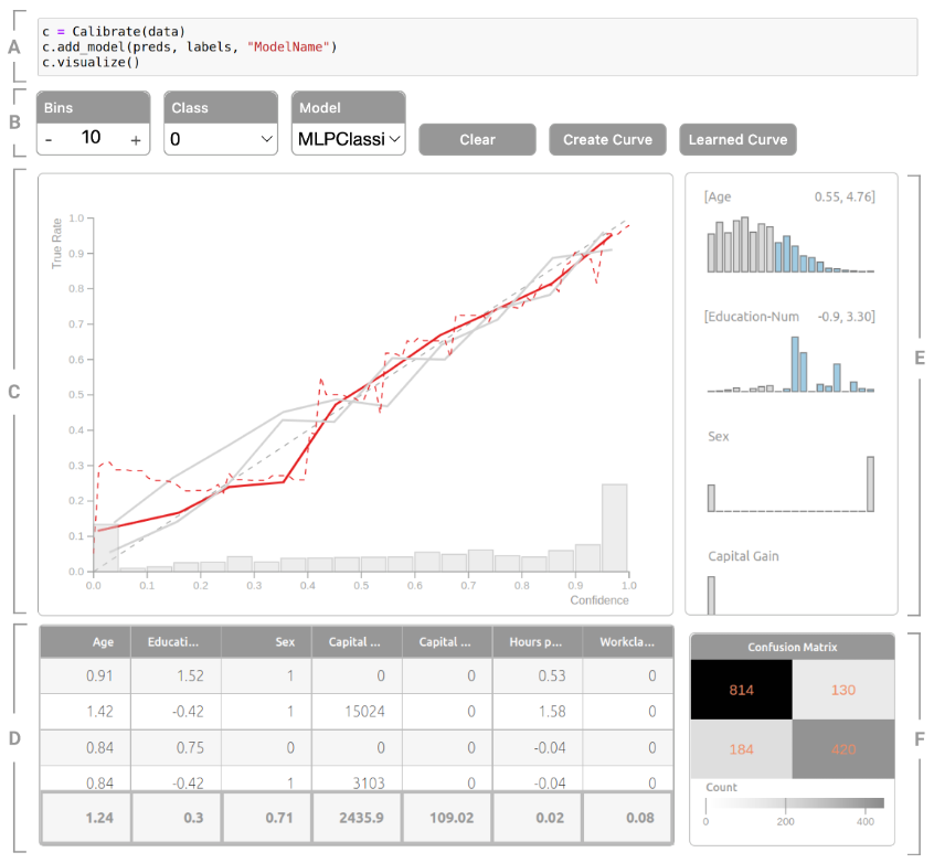{.nostretch width="50%" fig-align="center"} :::footer Xenopoulos, P., Rulff, J., Nonato, L. G., Barr, B., & Silva, C. (2022). [*Calibrate: Interactive analysis of probabilistic model output*](../refs/Xenopoulos_Rulff_Nonato_Barr_Silva_2022_Calibrate_Interactive_Analysis_Probabilistic_Output.pdf). IEEE TVCG. ::: ::: {.notes} Calibrate, from our group, TVCG. Letters follow the caption. A: it is one line in a Jupyter notebook. B: controls for bins, class and model. C: the calibration view, with a conventional binned reliability curve in solid and the learned reliability diagram as the red dashed line, over a histogram of predictions so you can see where the curve is supported. D: the instance view, populated by brushing a region of the calibration view. E: the feature view, histograms per feature, where brushing a range defines a subgroup, here a range of age and education, and its curve is drawn against the full population. F: a confusion matrix for the brushed region. The task is income prediction on Census data. The argument: calibration is rarely uniform, a model can be calibrated overall and badly off for a subgroup, and you only find that interactively. ::: ## Calibrate (2023) - Learned Reliability Diagram {fig-align="center"} :::footer Xenopoulos, P., Rulff, J., Nonato, L. G., Barr, B., & Silva, C. (2022). [*Calibrate: Interactive analysis of probabilistic model output*](../refs/Xenopoulos_Rulff_Nonato_Barr_Silva_2022_Calibrate_Interactive_Analysis_Probabilistic_Output.pdf). IEEE TVCG. ::: ::: {.notes} Our answer to the binning problem. Left: conventional diagrams for a random forest on Wisconsin breast cancer, 8 bins dotted and 10 bins solid. Two more bins and the curve changes shape completely, with a spike to 1.0 near 0.7. The rug along the bottom shows why: almost no predictions fall in the middle. Right: the learned reliability diagram. Instead of binning, fit a model that predicts the label from the predicted probability and plot that function. We use an Explainable Boosting Machine, and the three curves are max_bins of 50, 100 and 200: they nearly coincide. ECE is then the area between the curve and the diagonal. Same idea as the calibration maps two slides back, used for diagnosis rather than correction. ::: ## Calibrate (2023) ::: {style="display: flex; justify-content: center;"} ::: :::footer Xenopoulos, P., Rulff, J., Nonato, L. G., Barr, B., & Silva, C. (2022). [*Calibrate: Interactive analysis of probabilistic model output*](../refs/Xenopoulos_Rulff_Nonato_Barr_Silva_2022_Calibrate_Interactive_Analysis_Probabilistic_Output.pdf). IEEE TVCG. ::: ::: {.notes} Four-minute video of Calibrate in use: loading a model, reading the learned curve, brushing features to define subgroups, inspecting instances. It is a local file, so it plays without the network. If time is short, show the subgroup brushing part and skip the rest. ::: ## Smooth ECE (2023) {fig-align="center"} :::footer Błasiok, J., & Nakkiran, P. (2023). *Smooth ECE: Principled Reliability Diagrams via Kernel Smoothing*. arXiv preprint arXiv:2309.12236. ::: ::: {.notes} Błasiok and Nakkiran, 2023, a second answer to binning, from the theory side. Left: a binned reliability diagram with 15 bins, shaded by bin population, ECE 0.161. Right: the same predictions as a kernel regression of the label on the prediction. The red curve's thickness encodes the density of predictions, so you see where the curve has support, and the grey band is a bootstrapped confidence interval. smECE is 0.138 plus or minus 0.016: the metric comes with an error bar. This model is a clean sigmoid, underconfident, which the binned version only hints at. The bandwidth is chosen by their theory rather than by the user, so there is no hyperparameter left to argue about. ::: ## Smooth ECE (2023) {fig-align="center"} :::footer Błasiok, J., & Nakkiran, P. (2023). *Smooth ECE: Principled Reliability Diagrams via Kernel Smoothing*. arXiv preprint arXiv:2309.12236. ::: ::: {.notes} How the smooth diagram is built. Left: predictions on a line, negatives drawn up in green and positives down in blue. Step 1: kernel density estimate for each class separately. Step 2: at each value of f, take a vertical slice and normalize: the blue fraction of the slice is the estimated probability of a positive given that prediction. The red dashed curve on the right is that fraction. It is a reliability diagram where every point borrows strength from its neighbours instead of being hard-assigned to a bin. Available as the relplot Python package. ::: ## Visualizing Calibration for Multi-Class Problems {fig-align="center"} :::footer Vaicenavicius, J., Widmann, D., Andersson, C., et al. (2019). [*Evaluating model calibration in classification*](../refs/Vaicenavicius_Widmann_Andersson_Lindsten_Roll_Schon_2019_Evaluating_Model_Calibration.pdf). AISTATS. ::: ::: {.notes} Calibration beyond binary. Vaicenavicius et al., AISTATS 2019. Reducing a multiclass model to its top-class confidence, as the Guo figure does, hides miscalibration among the other classes. Here a CIFAR-10 LeNet's ten classes are merged into three groups so that a prediction is a point in a triangle. Each small triangle is a bin, coloured by how many predictions fall in it, most are at the corners, and the arrow goes from the bin's mean prediction to its observed class frequencies. Long arrows mean miscalibration, and their direction says which class is over-predicted. Left 25 bins, right 100 bins, and the same binning sensitivity shows up again. It stops at three dimensions, which is the open problem. ::: ## Suggested Calibration Literature * Niculescu-Mizil, A., & Caruana, R. (2005). [Predicting good probabilities with supervised learning](../refs/Niculescu_Mizil_Caruana_2005_Predicting_Good_Probabilities_Supervised_Learning.pdf). ICML. * Nixon, J., Dusenberry, M. W., Zhang, L., Jerfel, G., & Tran, D. (2019, June). [Measuring Calibration in Deep Learning](http://openaccess.thecvf.com/content_CVPRW_2019/papers/Uncertainty%20and%20Robustness%20in%20Deep%20Visual%20Learning/Nixon_Measuring_Calibration_in_Deep_Learning_CVPRW_2019_paper.pdf). In CVPR Workshops (Vol. 2, No. 7). * Guo, C., Pleiss, G., Sun, Y., & Weinberger, K. Q. (2017). [On calibration of modern neural networks](../refs/Guo_Pleiss_Sun_Weinberger_2017_Calibration_Modern_Neural_Networks.pdf). ICML. * Vaicenavicius, J., Widmann, D., Andersson, C., Lindsten, F., Roll, J., & Schön, T. (2019, April). [Evaluating model calibration in classification](http://proceedings.mlr.press/v89/vaicenavicius19a/vaicenavicius19a.pdf). In The 22nd International Conference on Artificial Intelligence and Statistics (pp. 3459-3467). PMLR. ::: {.notes} This slide provides a list of important papers on calibration. The Niculescu-Mizil and Caruana paper is a classic in this area. One line on each, so they know which to read. Niculescu-Mizil and Caruana, 2005, is the empirical survey: it compares learning algorithms by the quality of their probabilities rather than their accuracy, and it is the paper Guo is answering, because it found that the neural networks of the time were well calibrated. Read it to see how differently each model family distorts its scores, and why Platt scaling exists. Nixon and colleagues, 2019, is the critical one: it takes ECE apart and shows how sensitive it is to the binning scheme, the number of bins and whether you measure the top class or all classes. If they only read one of these after today, and they were interested in the binning thread, this is it. Guo and colleagues, 2017, is the one we looked at, and it is the reason calibration is a deep learning topic. It documents the problem, explains it through depth, width, batch norm and weight decay, and proposes temperature scaling. Vaicenavicius and colleagues, 2019, is the statistical treatment: it shows that the usual estimators of calibration error are biased, that the bias depends on the number of bins and the sample size, and it introduces the multiclass view we see at the end of the section. Mention that the honest version of 'this model has ECE 0.03' needs a confidence interval, which almost no paper gives, and which Smooth ECE provides. ::: ## Suggested Calibration Literature * Kull, M., & Flach, P. (2015). [Novel decompositions of proper scoring rules for classification: Score adjustment as precursor to calibration](../refs/Kull_Flach_2015_Novel_Decompositions_Proper_Scoring_Rules.pdf). ECML-PKDD, pp. 68-85. * Silva Filho, T. et al. (2020). [ECML/PKDD 2020 Tutorial: Evaluation metrics and proper scoring rules](../refs/Silva_Filho_2020_ECML_PKDD_Tutorial_Evaluation_Metrics.pdf). Full tutorial at [classifier-calibration.github.io](https://classifier-calibration.github.io/). * [Google Colab notebook for calibration curves](https://colab.research.google.com/drive/1mqDVJICMBg2eoIr2VPaDjQFUzlDT3grc?usp=sharing) * Minderer, M. et al. (2021). [Revisiting the calibration of modern neural networks](https://arxiv.org/abs/2106.07998). NeurIPS. * Xenopoulos, P., Rulff, J., Nonato, L. G., Barr, B., & Silva, C. (2022). [Calibrate: Interactive analysis of probabilistic model output](../refs/Xenopoulos_Rulff_Nonato_Barr_Silva_2022_Calibrate_Interactive_Analysis_Probabilistic_Output.pdf). IEEE TVCG. * Błasiok, J., & Nakkiran, P. (2023). [Smooth ECE: Principled reliability diagrams via kernel smoothing](https://arxiv.org/abs/2309.12236). arXiv. Python package: `relplot` ::: {.notes} Where to go deeper. Kull and Flach is the source for the refinement and calibration decomposition, the result behind the claim that recalibration can only fix one of the two terms. The ECML-PKDD 2020 tutorial by Silva Filho, Song, Perello-Nieto, Kull and Flach is the source for this whole section of the lecture, and its website has the slides, videos and notebooks; the forecast example and the reliability diagrams we walked through come from there. The Colab notebook reproduces the reliability diagrams from today, and it is the fastest way to start on a project that touches calibration. The last three are the papers behind the systems we saw at the end: Minderer and colleagues revisiting Guo's conclusion on modern architectures, our own Calibrate, and Blasiok and Nakkiran's Smooth ECE, whose relplot package will give them a reliability diagram with an error bar in one line. :::