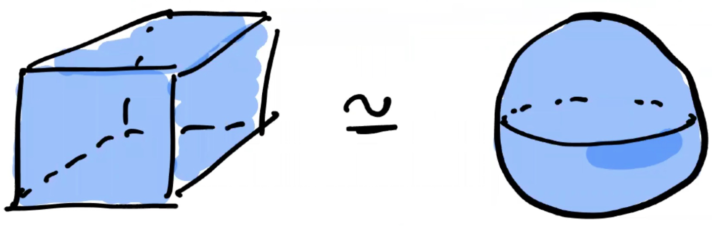
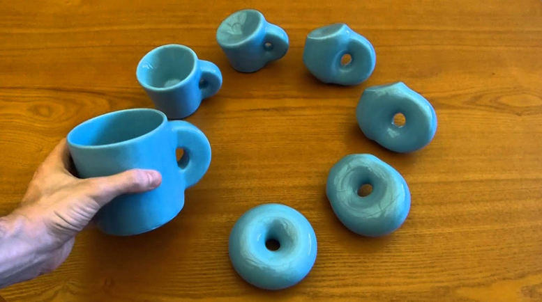
Topology studies the shape of mathematical objects
Unlike Geometry, it is not concerned with sizes, angles, nor coordinates
It is concerned with the connectivity (or lack of) between different “parts” of the object
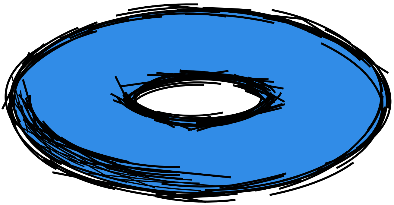
Two objects are topologically equivalent if we can transform one into another with continuous transformations (without tearing the object)
What is topology?
Why topology?
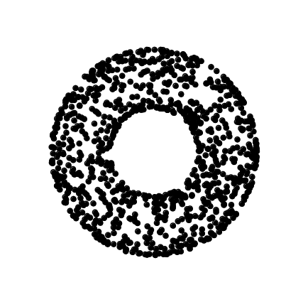
Since topology analyzes the shape while discarding possibly unnecessary information, it is frequently used for analyzing high-dimensional objects
Topological data analysis (TDA) uses techniques from topology to analyze datasets
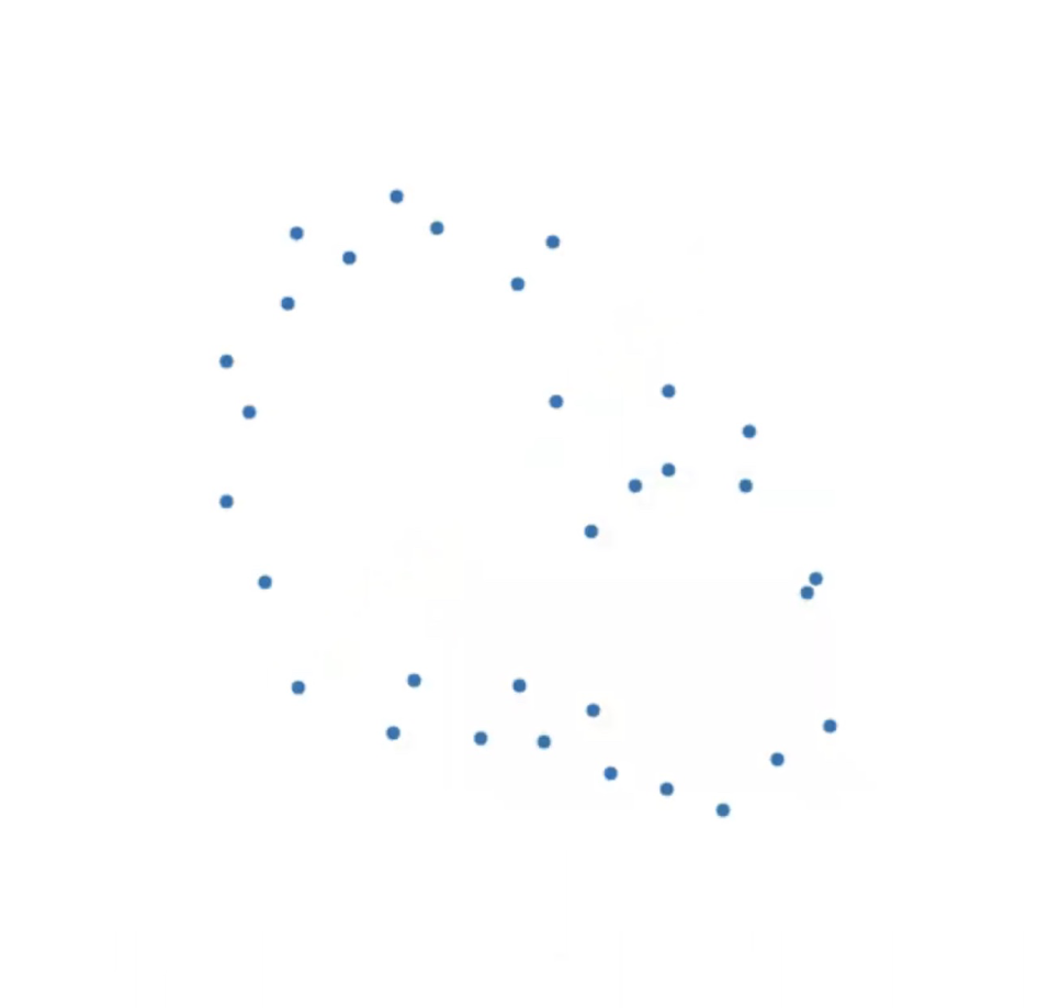
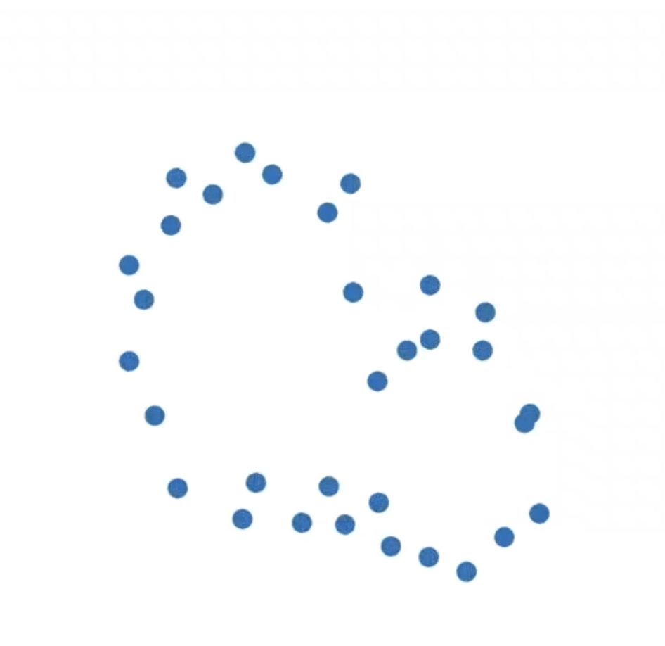
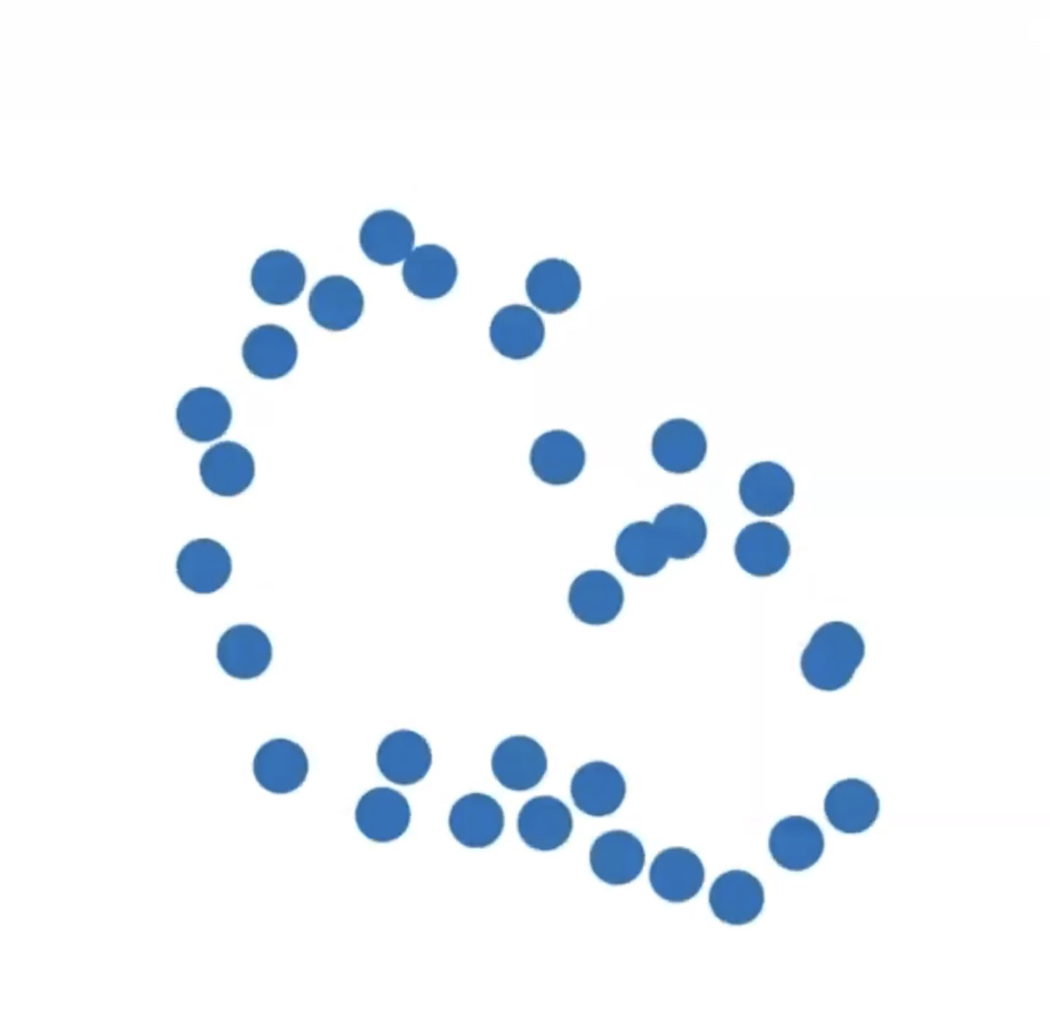
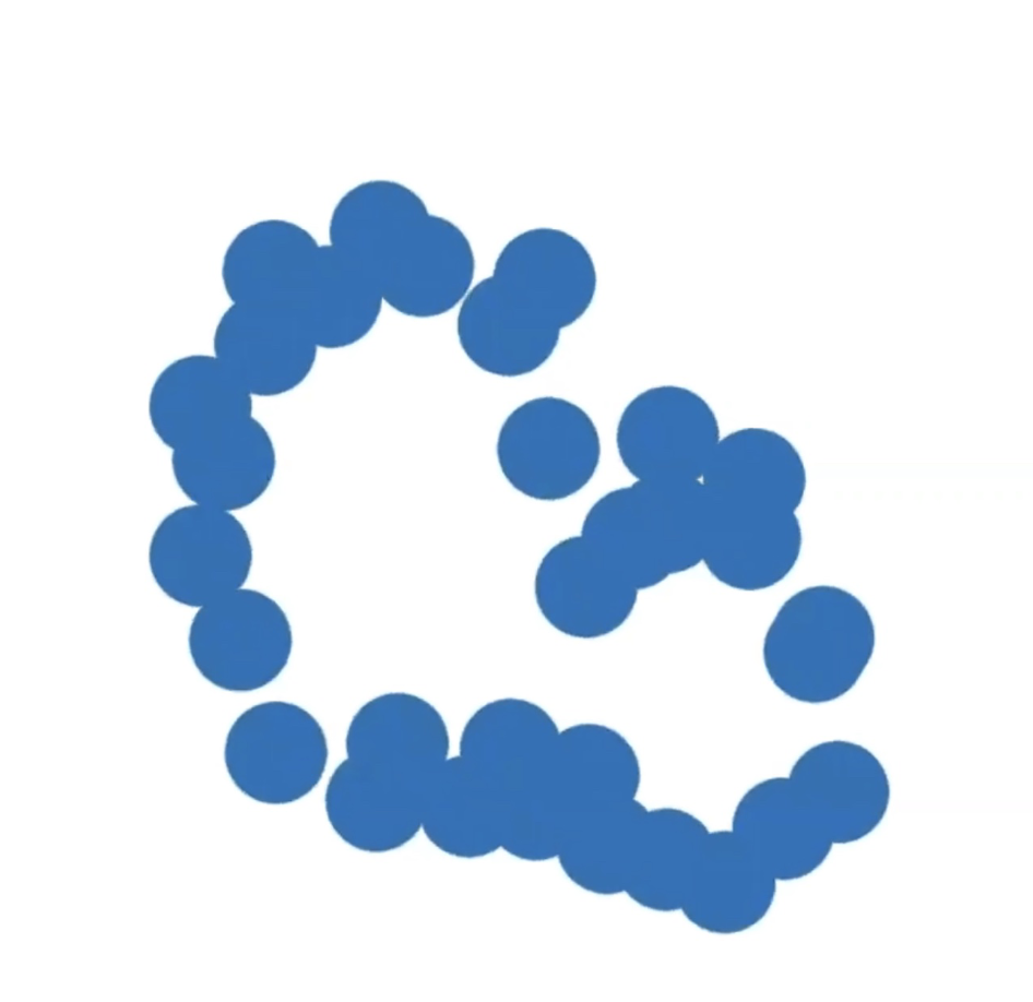
To do this, it is necessary to construct topological representations of the dataset’s points
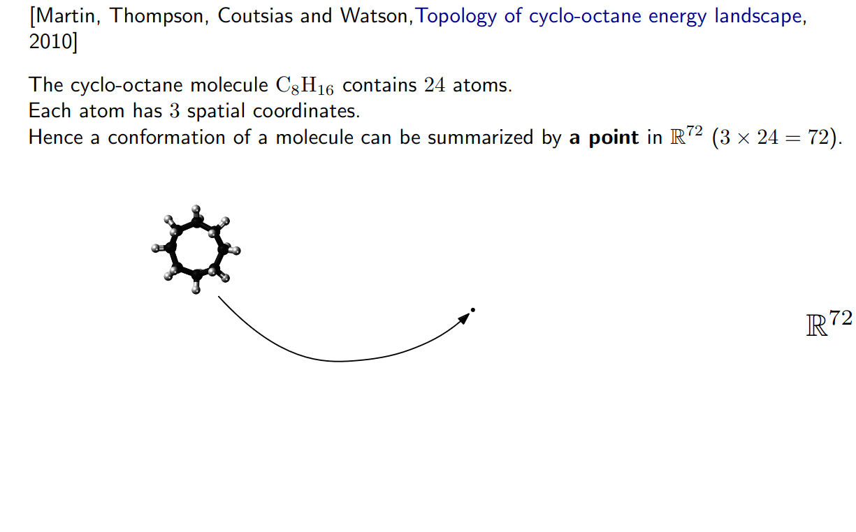
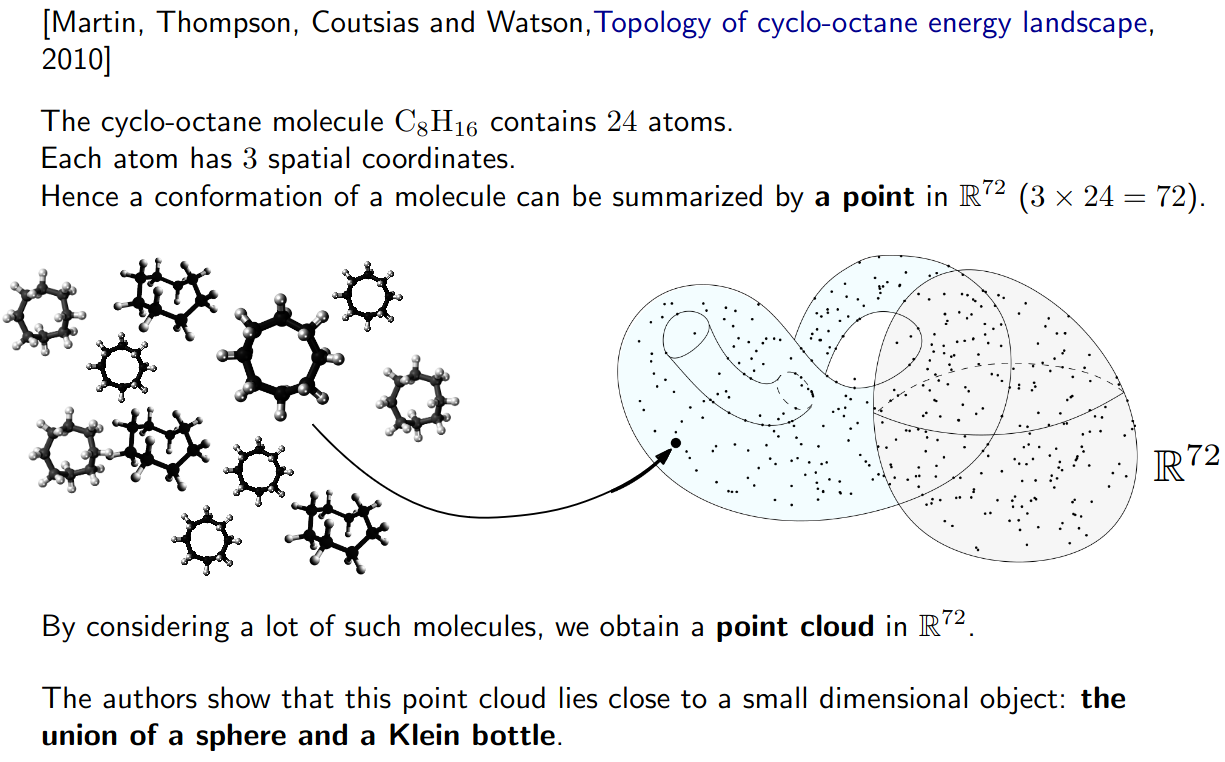
Why topology? - An example in chemistry
Why topology? - An example in chemistry
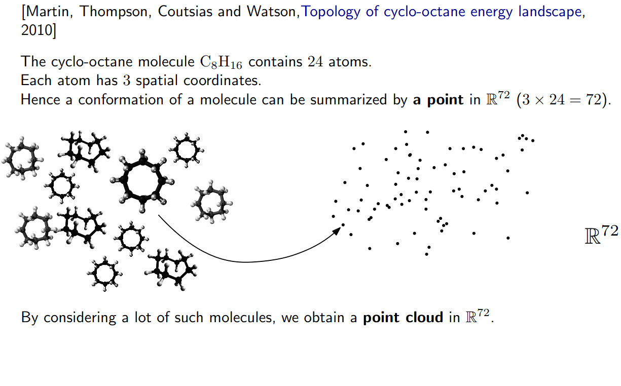
Why topology? - An example in chemistry
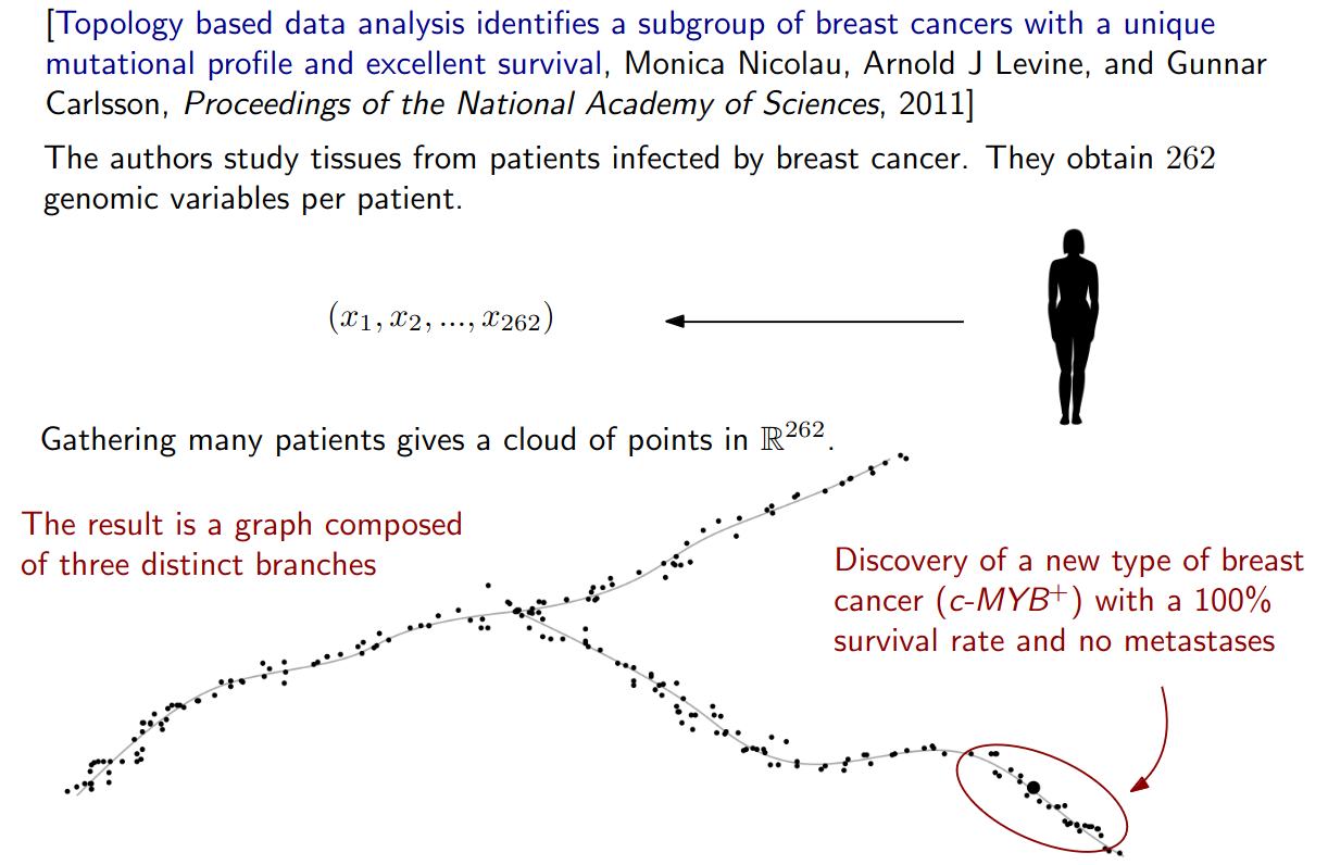
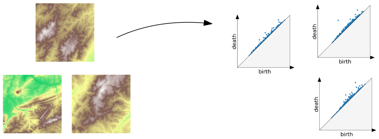
Why topology? - An example in biology
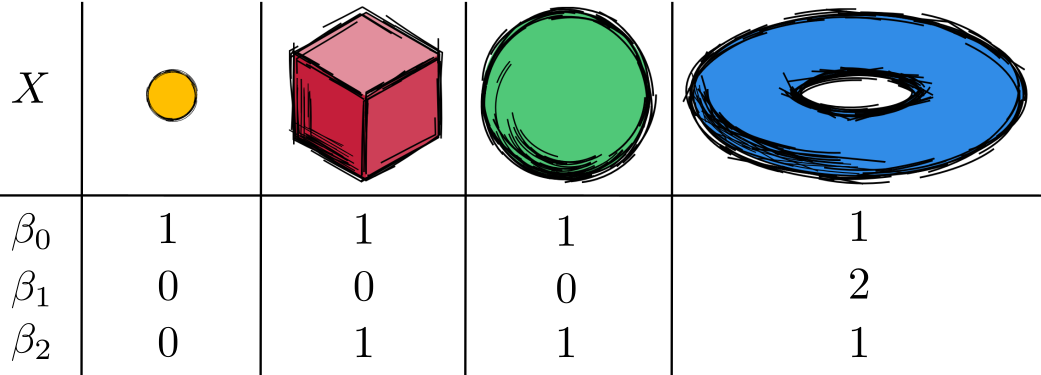
Betti numbers
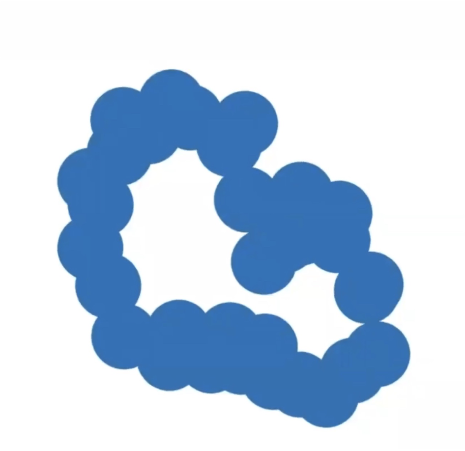
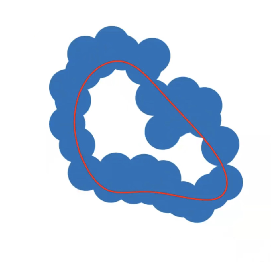
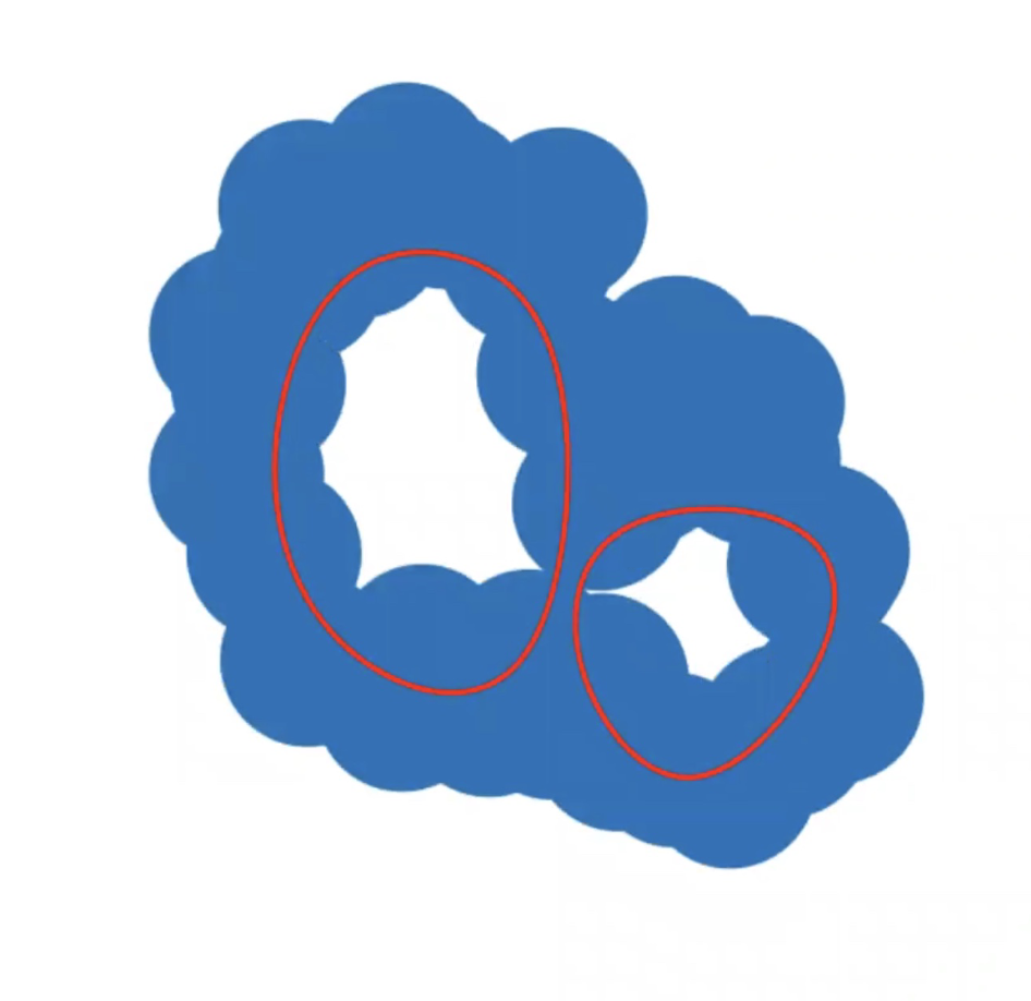
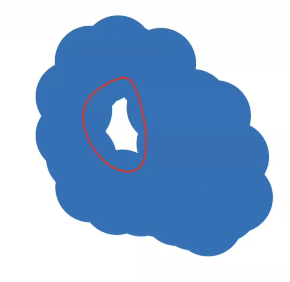
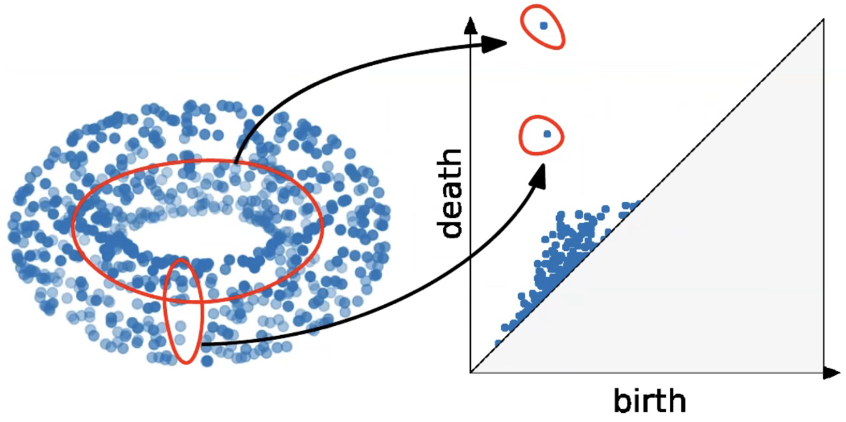
The \(d^{th}\) Betti number counts the number of \(d\)-dimensional holes. It can be used to distinguish between spaces.
\(\beta_0(X)\) Connected components in X
\(\beta_1(X)\) Tunnels or holes in X
\(\beta_2(X)\) Voids in X
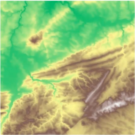
First Example - Map
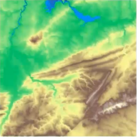
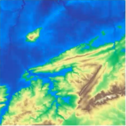
What is a peak?
First Example - Map
What is a peak?
First idea: Using local maximum
First Example - Map
What is a peak?
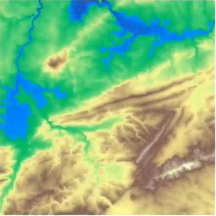
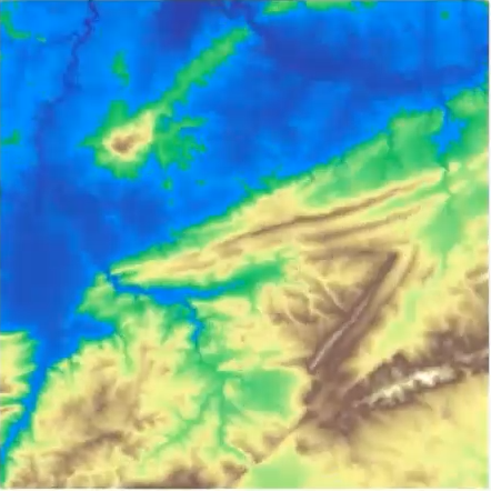
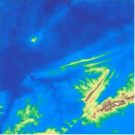
Second idea: flooding
First Example - Map
What is a peak?
Second idea: flooding
First Example - Map
What is a peak?
Second idea: flooding
First Example - Map
What is a peak?
Second idea: flooding
First Example - Map
What is a peak?
Second idea: flooding
First Example - Map
What is a peak?
Second idea: flooding
First Example - Map
What is a peak?
Second idea: flooding
First Example - Map
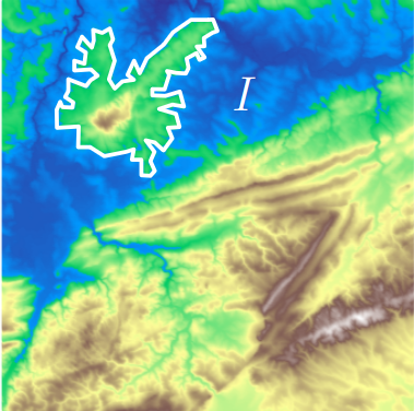
The island \(I\) appears at sea level \(b\) (its birth time)…
First Example - Map
The island \(I\) appears at sea level \(b\) (its birth time)…
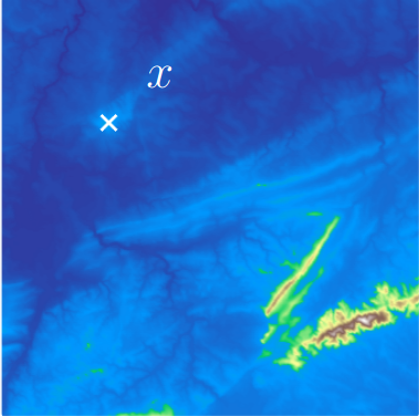
and disapears at seas level \(d\) (its death time) at local maximum \(x\).
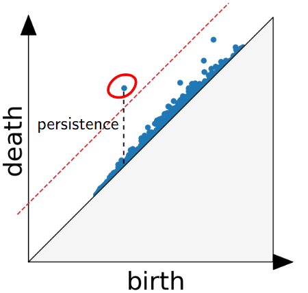
The point \(x\) is a peak if the persistence\(:= d-b\) of the island \(I\) is larger than \(91\)m (=\(300\)ft).
First Example - Map
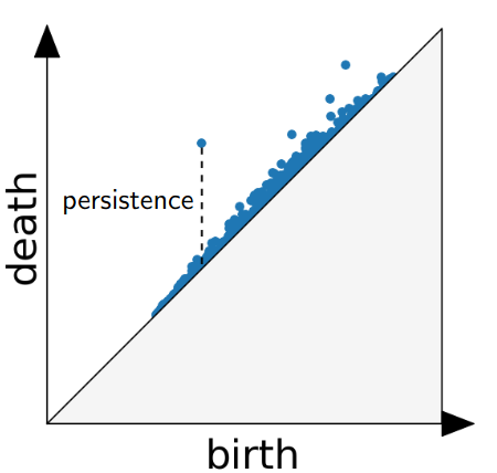
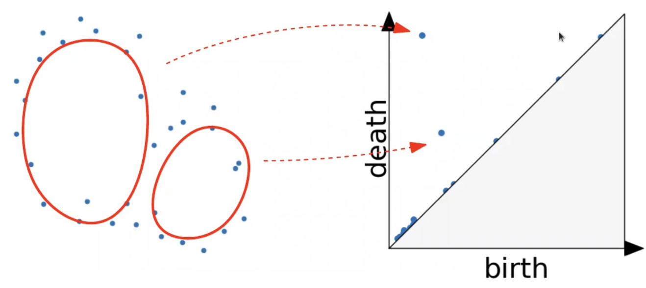
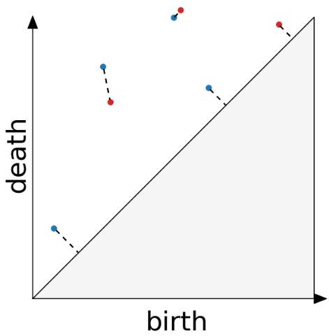
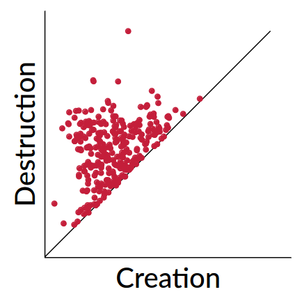
The persistence diagram (PD) of the elevation function is the collection of the points \((b,d)\), where \((b,d)\) corresponds to the birth/death of an island.
First Example - Map
The persistence diagram (PD) of the elevation function is the collection of the points \((b,d)\), where \((b,d)\) corresponds to the birth/death of an island.
Second Example
Second Example
Second Example
Second Example
Second Example
Second Example
Second Example
Second Example
Second Example
Second Example
Second Example
Second Example
Second Example
Persistence diagram
Distance between persistence diagrams
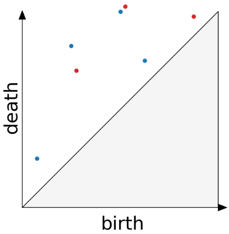
If we have more than one persistence diagram, how do we measure the distance between them?
Distance between persistence diagrams
We place both in the same diagram
Distance between persistence diagrams
We place both in the same diagram
Get the optimal pair matching between the points (including the diagonal)
Distance between persistence diagrams
We place both in the same diagram
Get the optimal pair matching between the points (including the diagonal)
The bottleneck distance between them will be the largest pair distance
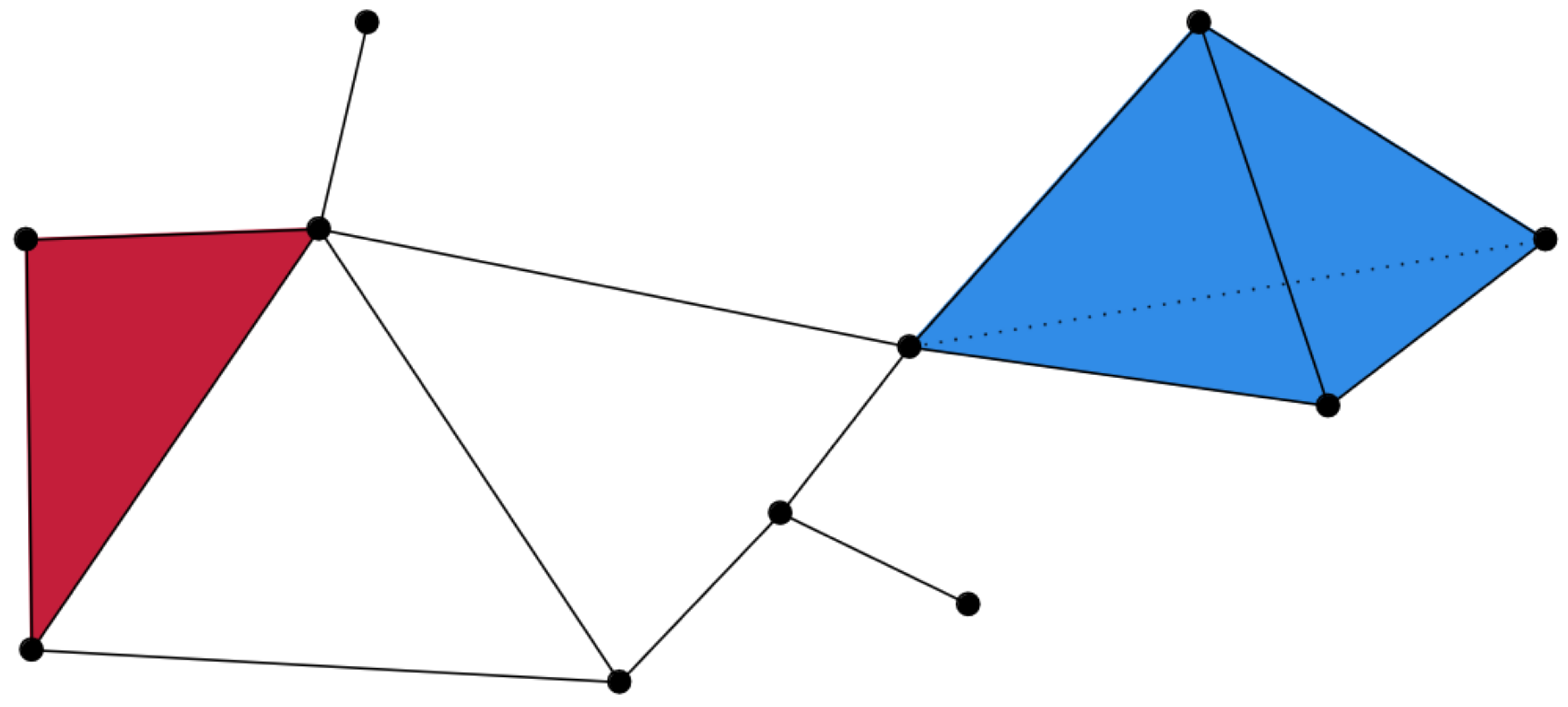
Simplicial complexes
Definition
We call a non-empty family of sets \(K\) with a collection of non-empty subsets \(S\) an abstract simplicial complex if:
\(\{v\} \in S\) for all \(v \in K\)
If \(\sigma \in S\) and \(\tau \subseteq \sigma\), then \(\tau \in K\).
Terminology
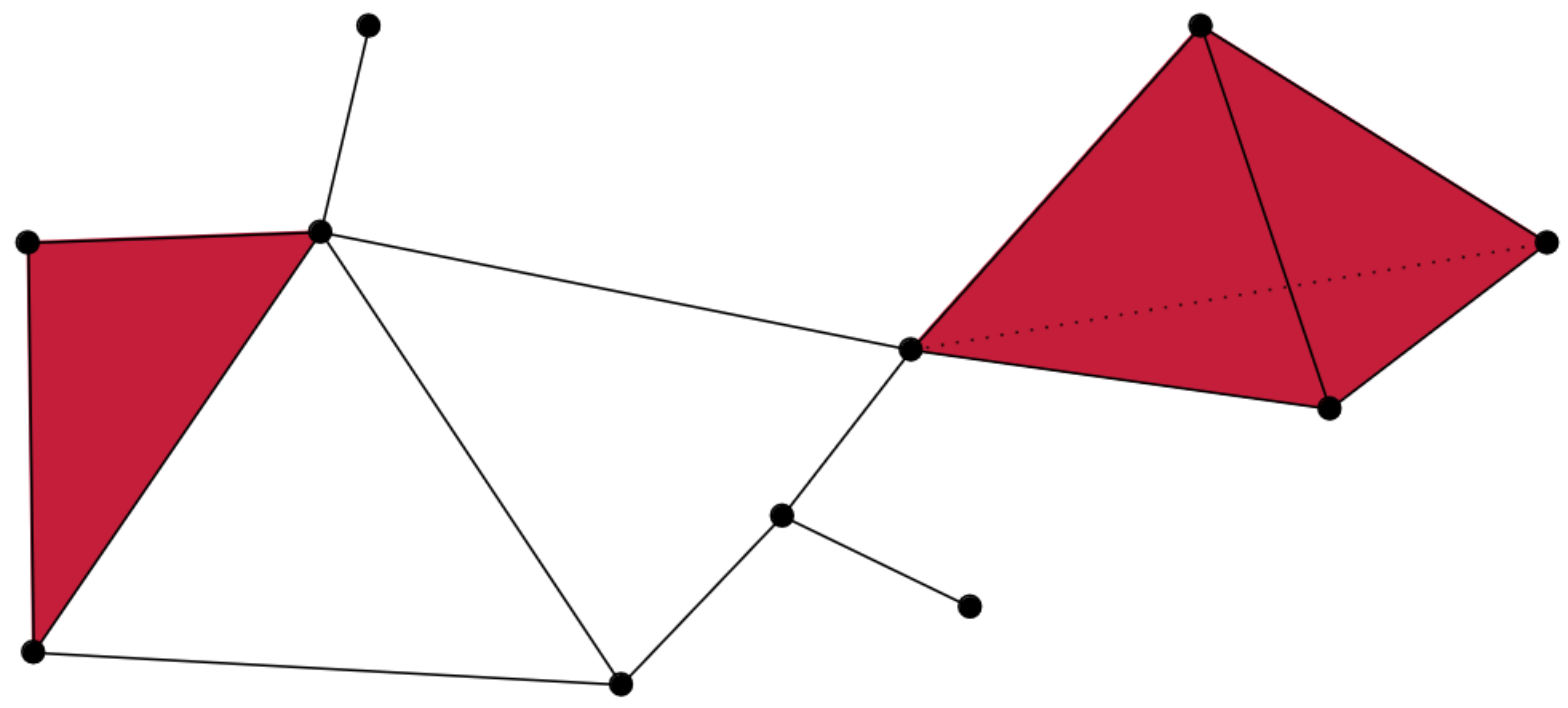
The elements of a simplicial complex \(K\) are called simplices. A \(k\)-simplex consists of \(k+1\) verticies.
Simplicial complexes
Example
Simplicial complexes can be decomposed into their skeletons, which only contain simplices of a certain dimension.
Simplicial complexes
Example
Simplicial complexes can be decomposed into their skeletons, which only contain simplices of a certain dimension.
Simplicial complexes
Example
Simplicial complexes can be decomposed into their skeletons, which only contain simplices of a certain dimension.
Simplicial complexes
Example
Simplicial complexes can be decomposed into their skeletons, which only contain simplices of a certain dimension.
Simplicial complexes
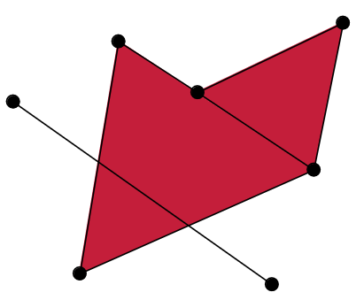
Non-example
This is not a simplicial complex because some higher-dimensional simplices do not intersect in a lower dimensional one!
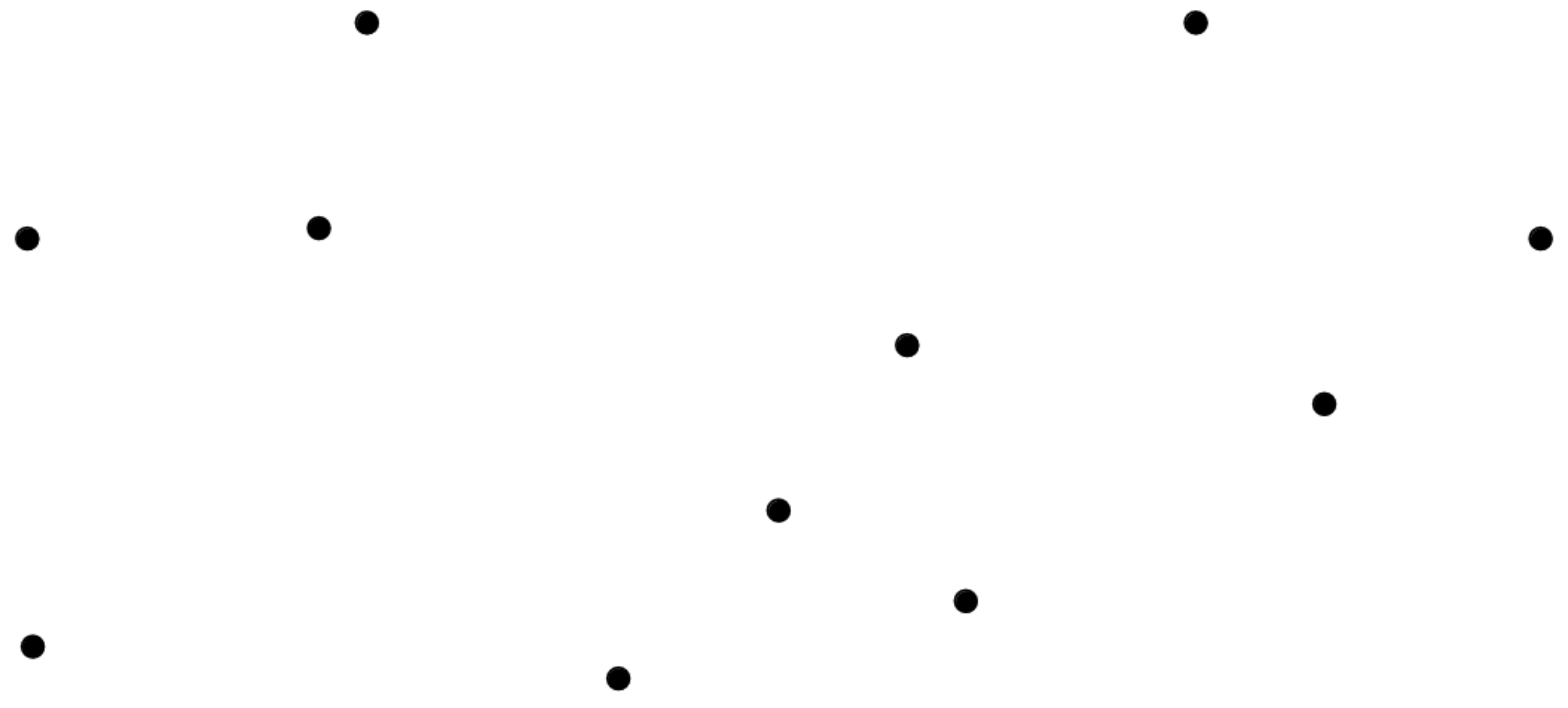
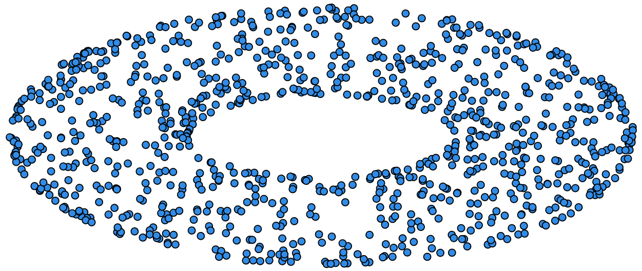
From points clouds to simplicial complexes
From points clouds to simplicial complexes
From points clouds to simplicial complexes
Strategy 1: Triangulation
Constructing the data’s simplicial complex
Vietoris-Rips construction
Definition
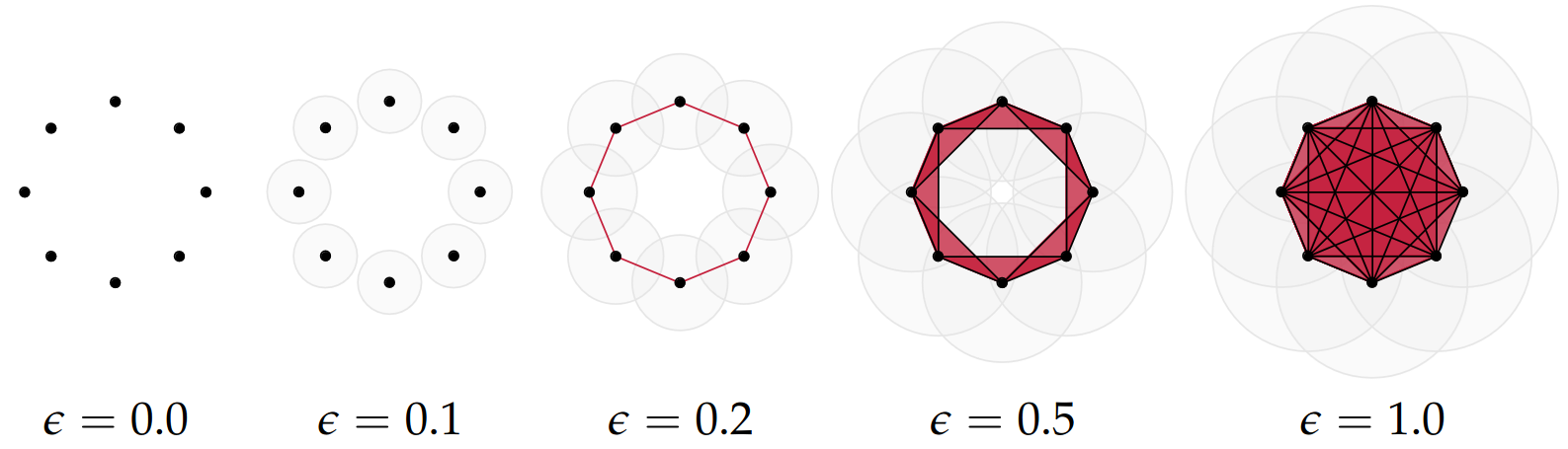
Given a set of points \(\mathcal{X} = \{x_1,\dots,x_n\}\) and a metric \(dist\) (such as the Euclidean distance), pick a threshold \(\epsilon\) and build the Vietoris-Rips complex \(\mathcal{V}_\epsilon\) defined as:
Equivalently, \(\mathcal{V}_\epsilon\) contains all simplices whose diameter is less than or equal to \(\epsilon\).
Vietoris-Rips construction
Example
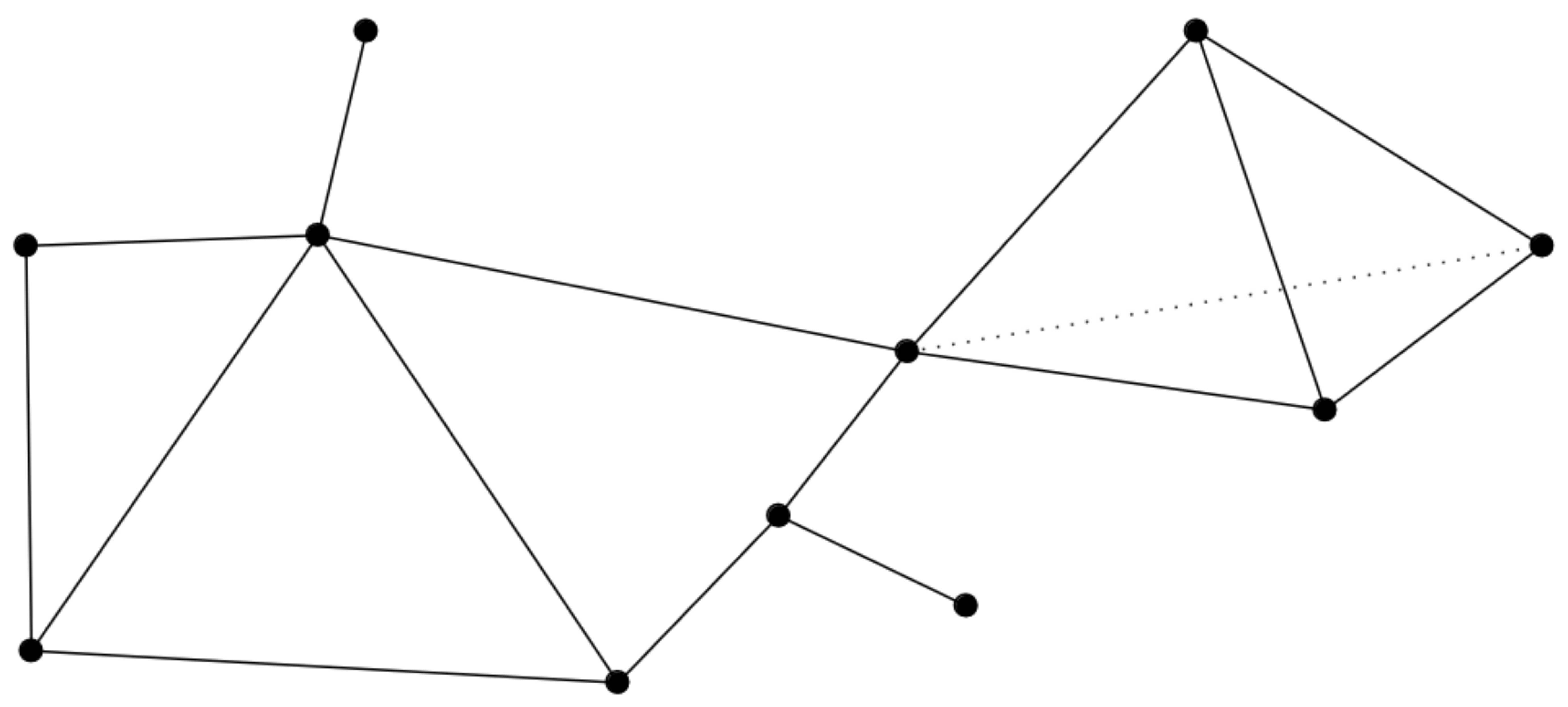
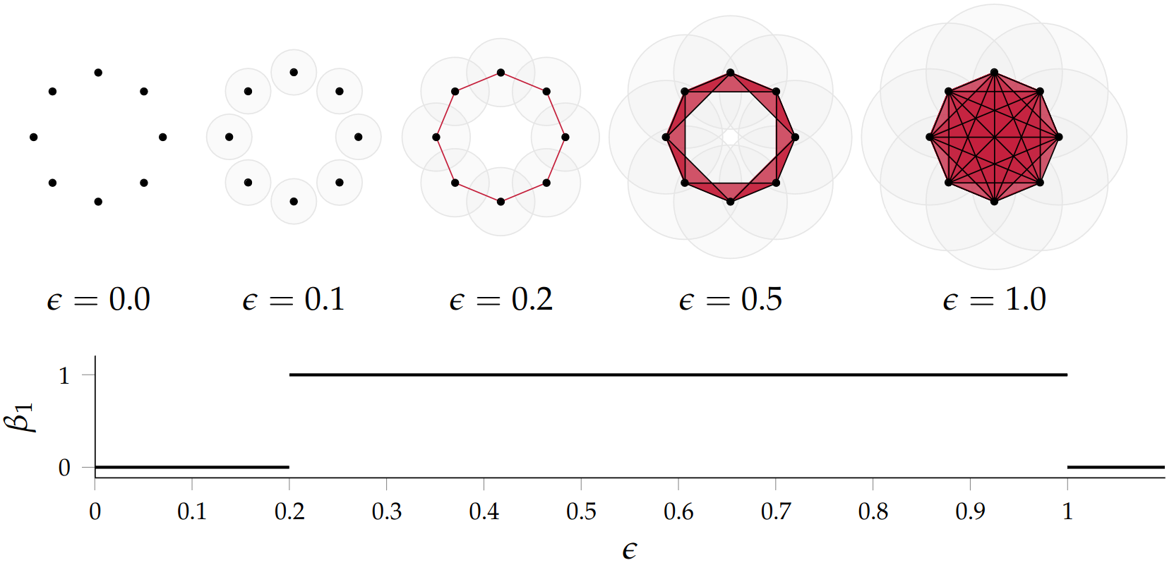
Draw Euclidean circles of diameter \(\epsilon\) and create a \(k\)-simplex \(\sigma\) for each subset of \(k+1\) points that intersect pairwise.
Some details about this construction
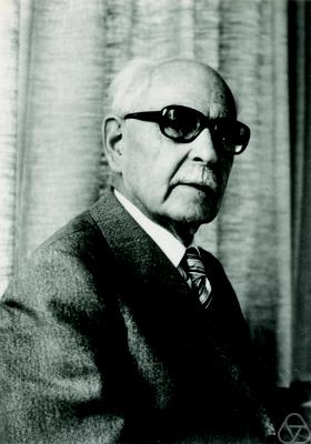
This construction dates back to a 1927 article by Leopold Vietoris\(^1\)
A 2010 paper by Afra Zomorodian\(^2\) describes several construction algorithms
The basic idea is to build higher-dimensional simplices inductively from lower-dimensional ones
In the worst case, the Vietoris-Rips complex will contain all \(2^n\) subsets of its underluing point clous \(\mathcal{X}\)!
The betti numbers of a Vietoris-Rips complex
Example
Issues with this approach
How to pick \(\epsilon\)?
There might not be one ‘correct’ value for \(\epsilon\).
Computationally inefficient
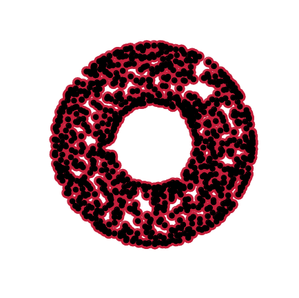
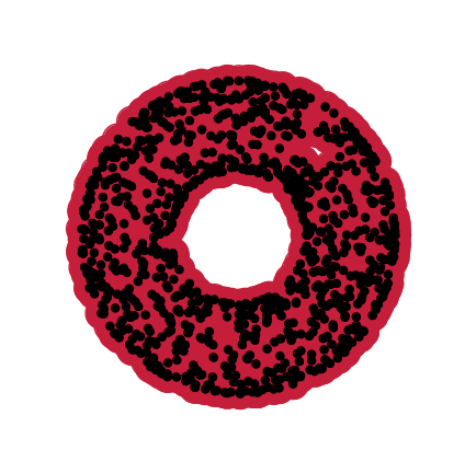
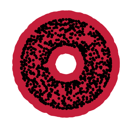
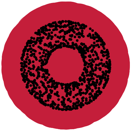
Picking \(\epsilon\) - Topological Persistence
Intuition: Go through all scales and track the topological features
Picking \(\epsilon\) - Topological Persistence
Intuition: Go through all scales and track the topological features
Picking \(\epsilon\) - Topological Persistence
Intuition: Go through all scales and track the topological features
Picking \(\epsilon\) - Topological Persistence
Intuition: Go through all scales and track the topological features
Picking \(\epsilon\) - Topological Persistence
Intuition: Go through all scales and track the topological features
Persistent homology
A filtration is a growing sequence of complexes: \(\mathcal{V}_{\epsilon_1} \subseteq \mathcal{V}_{\epsilon_2} \subseteq \cdots\) for \(\epsilon_1 \leq \epsilon_2 \leq \cdots\)
Homology is the machinery that counts the holes (the Betti numbers) of each complex
Persistent homology tracks every hole through the filtration: born at \(b\), dead at \(d\)
The output is a persistence diagram, one point \((b,d)\) per feature, with persistence \(= d-b\)
Same recipe on the map: the filtration is the sea level instead of \(\epsilon\)
Strategy 2: Data skeleton
The Mapper Algortihm
Math World
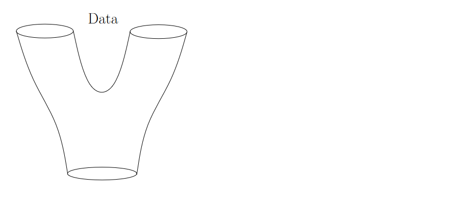
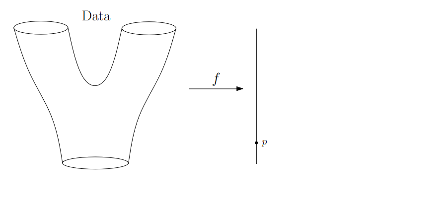
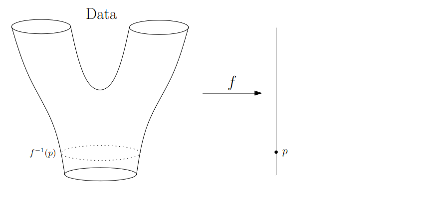
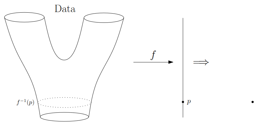
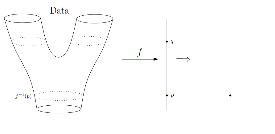
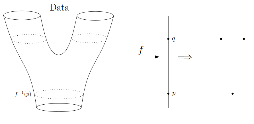
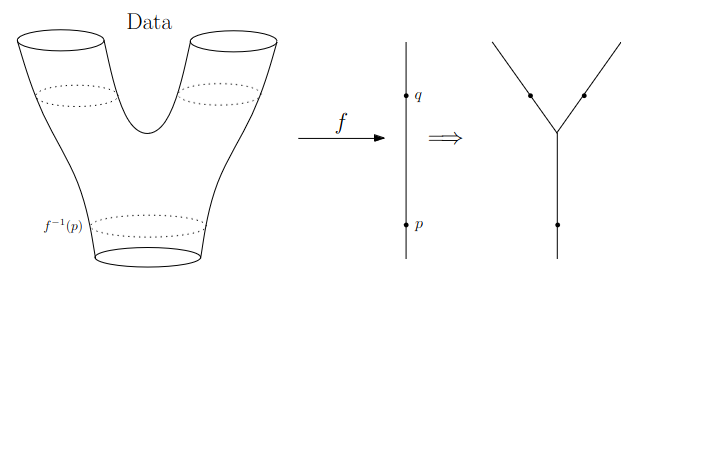
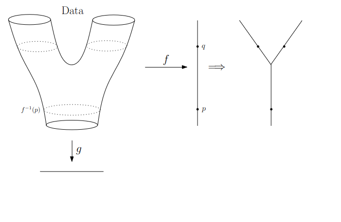
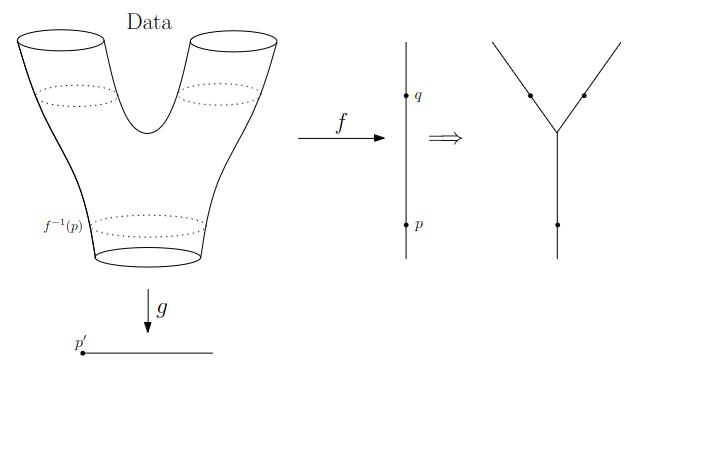
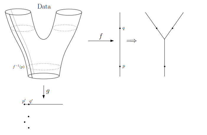
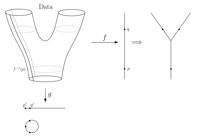
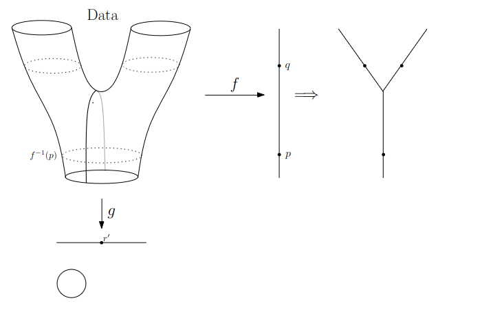
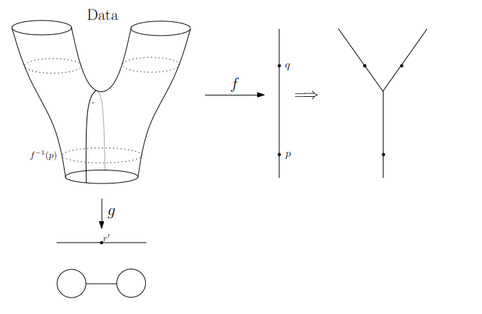
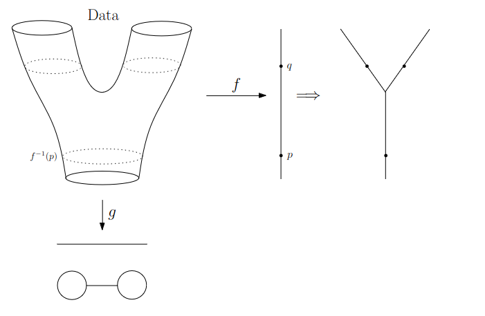
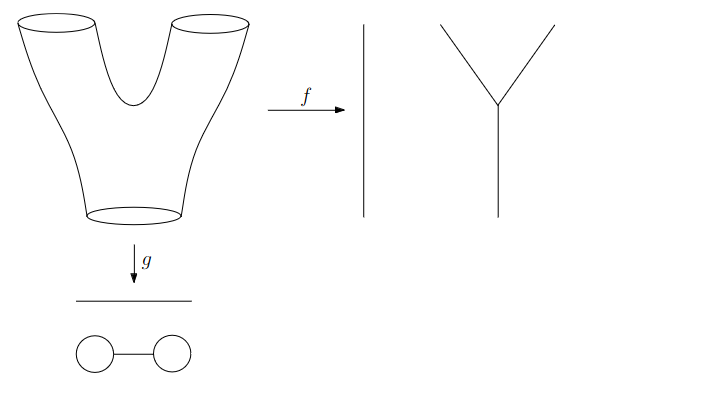
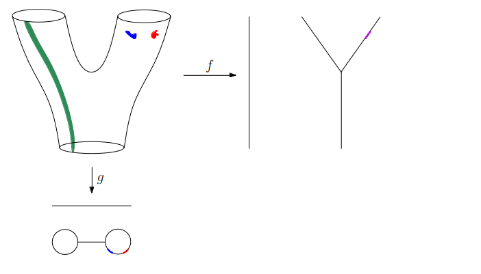
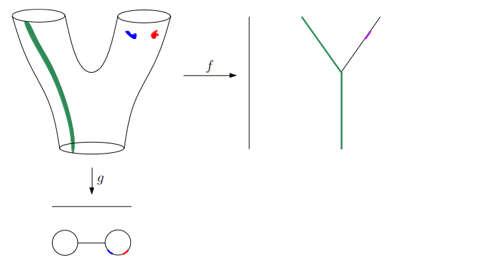
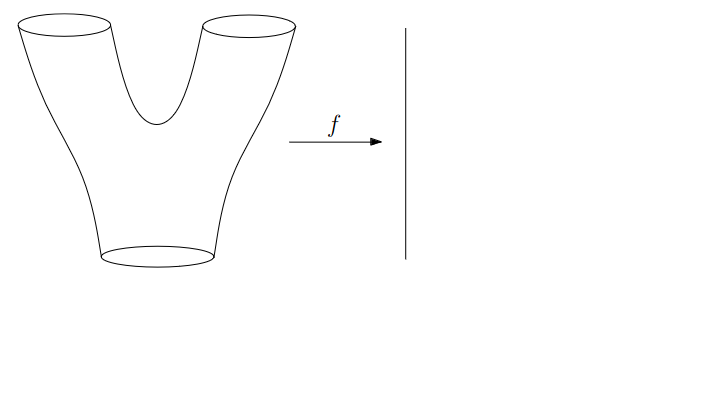
We start in “Math World”, where
We draw the data as a smooth manifold
Functions that appear are smooth or continuous
We will not need either of these assumptions once we are in the “Data World”.
Even more importantly, data in the real world is never like this.
Math World
Math World
Math World
Math World
Math World
Math World
Math World
Math World
Math World
Math World
Math World
Math World
Math World
Math World
Why is this useful?
We get “easy” understanding of the localizations of quantities of interest.
Why is this useful?
We get “easy” understanding of the localizations of quantities of interest.
Why is this useful?
We get “easy” understanding of the localizations of quantities of interest.
Why is this useful?
We get “easy” understanding of the localizations of quantities of interest.
Why is this useful?
We get “easy” understanding of the localizations of quantities of interest.
Why is this useful?
We get “easy” understanding of the localizations of quantities of interest.
Why is this useful?
We get “easy” understanding of the localizations of quantities of interest.
Why is this useful?
We get “easy” understanding of the localizations of quantities of interest.
Lenses inform us where in the space to look for phenomena.
For easy localizations many different lenses will be informative.
For hard (= geometrically distributed) localizations we have to be more careful. But even then, we frequently get incremental knowledge from a poorly chosen lens.
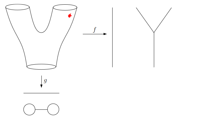
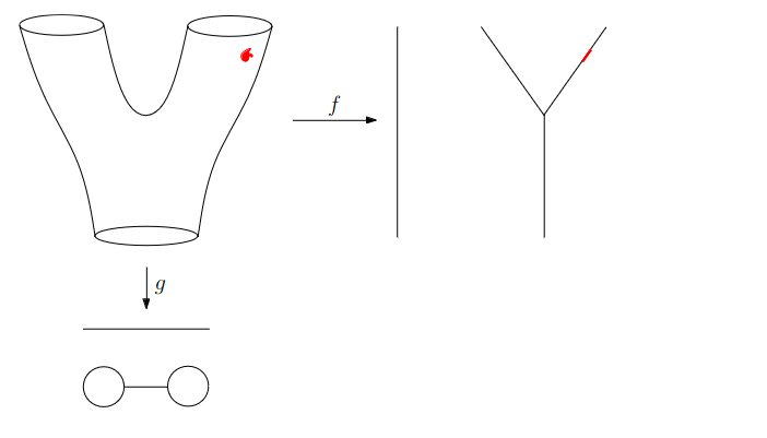
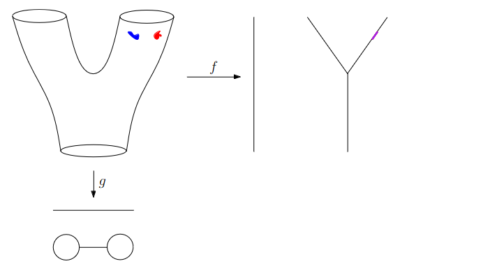
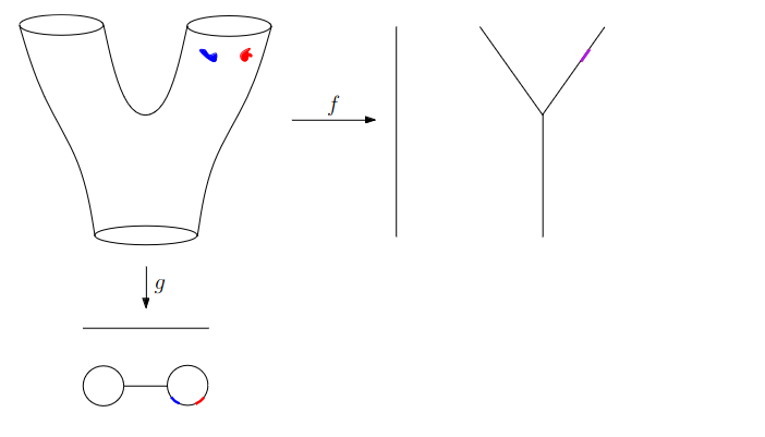
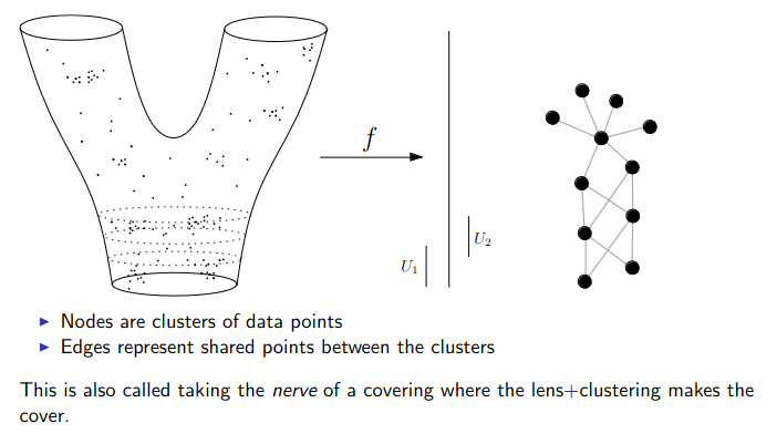
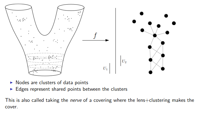
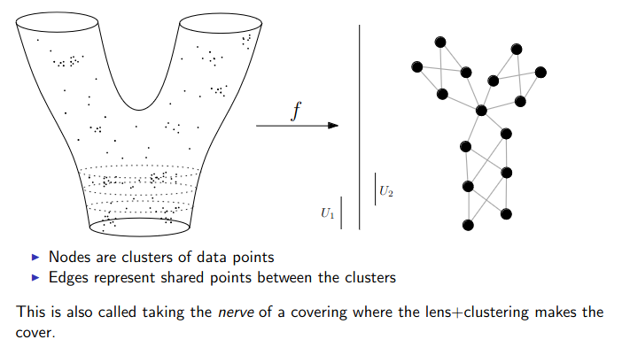
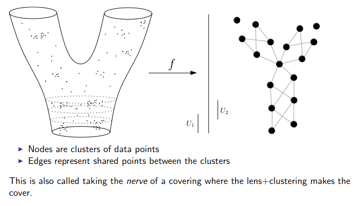
Data World - Mapper
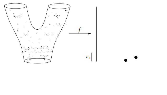
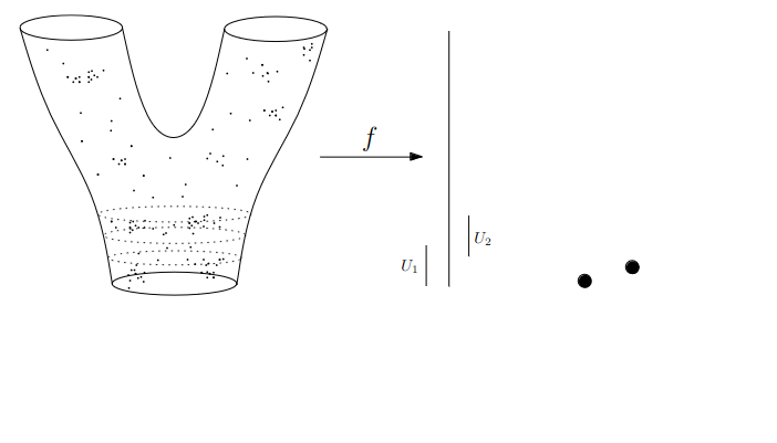
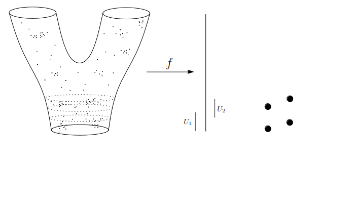
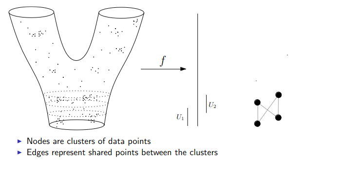
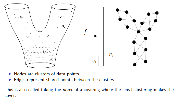
We need to adjust the “Math World” view to bring the algorithm into the “Data World”
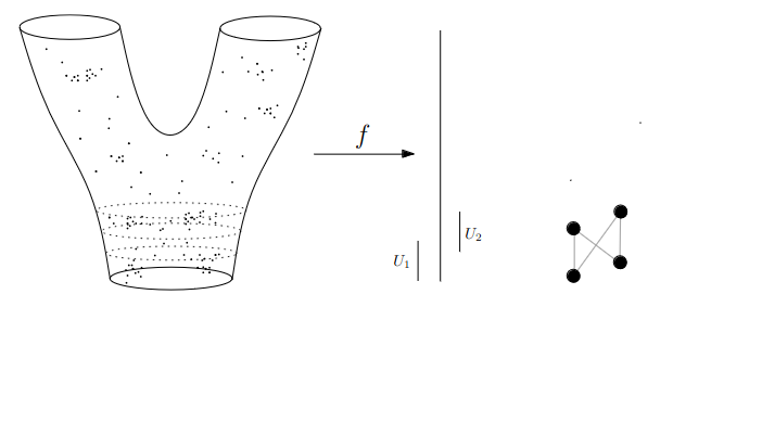
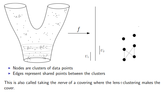
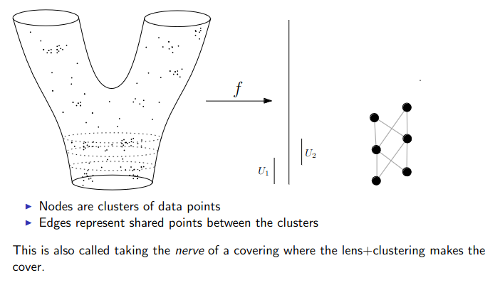
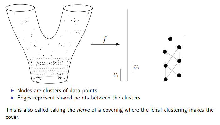
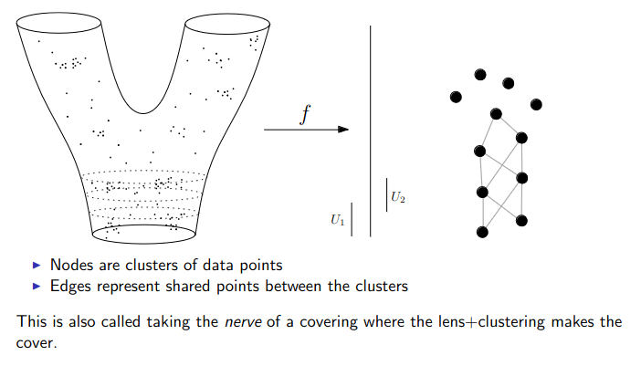
We replace points with open sets in the range of the lens
We replace “connected component of the inverse image” with “clusters in the inverse image”
We connect clusters (nodes) with an edge if they share points in common.
Data World - Mapper
Data World - Mapper
Data World - Mapper
Data World - Mapper
Data World - Mapper
Data World - Mapper
Data World - Mapper
Data World - Mapper
Data World - Mapper
Data World - Mapper
Data World - Mapper
Data World - Mapper
Data World - Mapper
Data World - Mapper
Data World - Mapper
Putting it together
Persistent homology
Mapper
Idea
Grow a complex across all scales
Cover the lens range, cluster, connect
Output
Persistence diagram
Graph (a skeleton of the data)
Tells you
How many pieces, loops, voids, and which are real
Branches, loops, where quantities concentrate
You choose
Metric, maximum dimension
Lens, intervals, overlap, clustering
In ML
Features and distances between diagrams
Exploring and visualizing complex data
TDA vs. t-SNE and UMAP
t-SNE / UMAP
TDA (persistence, Mapper)
Goal
Low-dimensional picture that keeps local neighborhoods
Summary of global shape: pieces, loops, voids, branches
Output
Points in the plane
Diagram or graph
Strength
Quick look at clusters
Quantifies structure, stable to small noise
Watch out
Layout, distances and cluster sizes can mislead, and depend on hyperparameters
Choice of lens or metric, cost on large data
Together: check whether an embedding kept the topology, or use an embedding coordinate as a Mapper lens.
Takeaways
Topology keeps connectivity and throws away exact geometry
In persistence, long-lived features are signal and short-lived ones are noise
In Mapper, the lens decides what you see, so try more than one
These summarize shape; they complement PCA, t-SNE and UMAP rather than replace them
Questions?
To look further
References
For more information about the persistence diagram, see Vincent Divol’s CDS Lunch Seminar presentation “Quantifying the topology of datasets using Topological Data Analysis”