
White-box Model Interpretation
Published:
Detect bias
Spot leakage] K --> K1[Learn patterns
Test hypotheses
Scientific insight] T --> T1[User confidence
Social acceptance
Stakeholder trust] C --> C1[Legal requirements
Fairness audits
Ethical guidelines] style MI fill:#2d3e50,stroke:#1f77b4,stroke-width:3px,color:#fff style D fill:#e74c3c,stroke:#c0392b,stroke-width:2px,color:#fff style K fill:#3498db,stroke:#2980b9,stroke-width:2px,color:#fff style T fill:#2ecc71,stroke:#27ae60,stroke-width:2px,color:#fff style C fill:#f39c12,stroke:#e67e22,stroke-width:2px,color:#fff style D1 fill:#ffebee,stroke:#c0392b,stroke-width:1px,color:#333 style K1 fill:#e3f2fd,stroke:#2980b9,stroke-width:1px,color:#333 style T1 fill:#e8f5e9,stroke:#27ae60,stroke-width:1px,color:#333 style C1 fill:#fff3e0,stroke:#e67e22,stroke-width:1px,color:#333 ``` --> ::: ::: ::: {.notes} Interpretability serves multiple critical functions. For debugging, we can catch issues like the model learning spurious correlations. For science, interpretable models reveal domain insights. For deployment, stakeholders need to trust the system. In regulated domains like healthcare and finance, interpretability may be legally required to justify decisions. ::: ## Machine-learning-assisted materials discovery using failed experiments ::: {.columns} ::: {.column width="40%"} 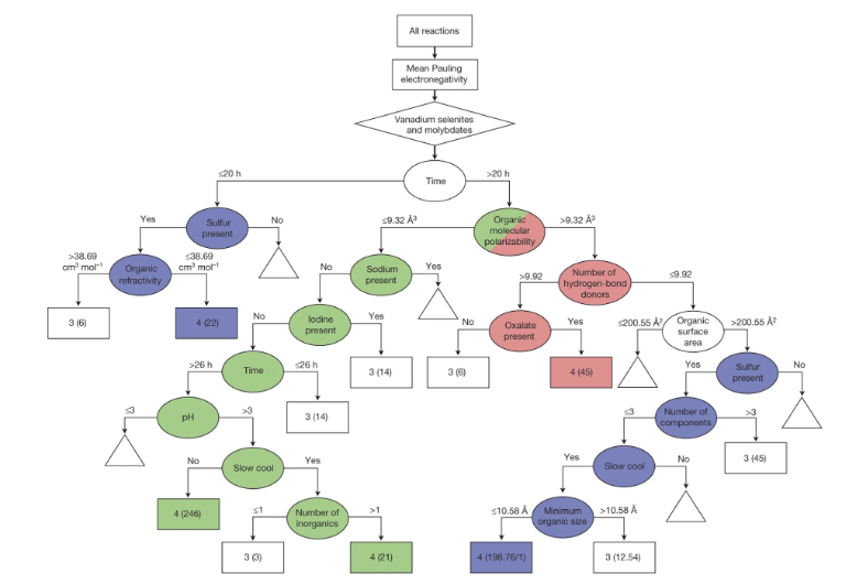 ::: ::: {.column width="60%"} - Researchers firstly built a database of chemistry experiments (new material). - Then they train an SVM to predict whether a new chemistry experiment will be successful. - Then they train a surrogate DT to explain the model to learn more about the experiment. ::: ::: ::: footer Raccuglia, P., et al. (2016). [Machine-learning-assisted materials discovery using failed experiments](https://doi.org/10.1038/nature17439). *Nature*, 533, 73-76. ::: ::: {.notes} This Nature paper demonstrates using interpretable models to understand scientific experiments. By training a surrogate decision tree on SVM predictions, researchers could extract human-understandable rules about which experimental conditions lead to success. ::: ## Properties of Good Explanations Human explanations are naturally: ::: {.incremental} 1. **Contrastive**: "Why this, rather than that?" (not exhaustive) - Example: "Loan denied because debt-to-income ratio was 45%, not the required ≤30%" 2. **Selective**: Focus on 1-3 key reasons (not all causes) 3. **Social**: Tailored to audience and context 4. **Focused on abnormal**: Highlight surprising factors 5. **Truthful but simple**: Balance accuracy with understandability ::: ::: footer Molnar, C. (2022). [*Interpretable Machine Learning*](https://christophm.github.io/interpretable-ml-book/interpretability.html). 2nd Edition. ::: ::: {.notes} Research on human explanations reveals important patterns. People don't want exhaustive causal chains - they want contrastive answers comparing to alternatives. Good explanations are selective, providing just a few key factors rather than everything. They should be tailored to the audience's knowledge and focus on surprising or abnormal causes rather than routine factors. This guides how we should design ML explanations. ::: ## Why Model Interpretation & Explanation? ::: {.columns} ::: {.column width="60%"} {width="700px"} ::: ::: {.column width="40%"} - Fairness - Privacy - Reliability or Robustness - Causality - Trust ::: ::: ::: {.notes} This paper highlights critical concerns in ML deployment. Fairness requires understanding if protected attributes influence decisions. Privacy needs transparency about what data influences predictions. Robustness demands knowing if the model relies on brittle features. Causality questions whether correlations are meaningful. All these build toward the ultimate goal: trust in AI systems. ::: ## Taxonomy of Interpretability Methods ::: {.columns} ::: {.column width="50%"} **Intrinsic (White-box)** - Interpretability built into model structure - Examples: Linear models, short decision trees, sparse models - Understand by examining model internals - *Today's focus* ::: ::: {.column width="50%"} **Post-hoc (Black-box)** - Explain after training - Works with any model (neural nets, ensembles) - Examples: LIME, SHAP, saliency maps - *Next week's topic* ::: ::: **Additional dimensions:** Model-specific vs Model-agnostic | Local vs Global | Feature importance vs Feature effects ::: footer [Christoph Molnar: Interpretable Machine Learning](https://christophm.github.io/interpretable-ml-book/taxonomy-of-interpretability-methods.html) ::: ::: {.notes} Intrinsic interpretability means the model structure itself is understandable - you can look at a decision tree and trace the logic. Post-hoc methods generate explanations after the fact for any model. We also distinguish: model-specific (works for one type) vs model-agnostic (works for any), local (explains one prediction) vs global (explains overall behavior), and feature importance (which features matter) vs feature effects (how do features influence predictions). Today we focus on intrinsically interpretable white-box models. ::: ## Outline - Model Interpretation and Explanation - White-box Approaches and Visualizations - Related Research in VIS & AI ## White-box Models We discuss the following models that are intrinsically interpretable: - Linear Regression - Generalized Additive Models (GAM) - Tree-based Models - Decision Rules ::: {.notes} These model families offer varying degrees of expressiveness and interpretability. Linear models are simplest but most limited; GAMs add non-linear flexibility; trees provide natural visual structure; rules offer explicit logic. ::: ## Linear Regression Linear models can be used to model the dependence of a regression target y on some features x in a format as below: \begin{equation} y = \beta_0 + \beta_1 x_1 + \ldots + \beta_n x_n + \varepsilon\end{equation} The predicted target $y$ is a linear combination of the weighted features $\beta_i x_i$. The estimated linear equation is a hyperplane in the feature/target space (a simple line in the case of a single feature). The weights specify the slope (gradient) of the hyperplane in each direction. ::: {.notes} Linear regression remains one of the most interpretable models. Each coefficient directly tells us how much the prediction changes when that feature increases by one unit, holding all else constant. This direct interpretability makes linear models valuable for policy decisions and scientific inference. ::: ## Linear Regression  ::: {.notes} This visualization shows the geometric interpretation of linear regression as fitting a hyperplane through the data points. The residuals (vertical distances from points to the plane) are minimized during training using least squares optimization. ::: ## Linear Regression: An Example of Housing Price  How do you interpret the influence of each property on the prediction of housing price? ::: {.notes} In this housing price model, we can directly read off the coefficients: each additional bedroom adds a certain amount to the price, each square foot contributes its value, proximity to schools has a measurable effect. The sign tells us direction (positive/negative), the magnitude tells us importance. This direct interpretability makes linear models valuable for explaining decisions to stakeholders. ::: ## Interpreting Linear Model Coefficients **Basic interpretation:** An increase in feature $x_j$ by one unit changes the prediction by $\beta_j$ units ::: {.incremental} - ✅ **Numerical features**: Direct marginal effect (holding others constant) - ✅ **Categorical features**: Coefficients show difference from reference category - ⚠️ **Scale-dependent**: Coefficients change with feature units - ⚠️ **"Holding others constant" assumes Feature Independence** (a strong assumption!) ::: ::: footer Molnar, C. (2022). [*Interpretable Machine Learning*](https://christophm.github.io/interpretable-ml-book/limo.html). Chapter 4.1. ::: ::: {.notes} The standard interpretation is deceptively simple: each coefficient tells you the marginal effect of that feature. But be careful - this interpretation assumes you can change one feature while holding others constant, which may not be realistic. For example, in housing, you can't easily change square footage without affecting other features. Coefficients are also scale-dependent - standardizing features helps comparisons. ::: ## Important Assumptions for Interpretation Linear models make strong assumptions: ::: {.incremental} 1. **Linearity**: Effects are additive (no interactions unless explicitly added) 2. **Independence**: Features are not strongly correlated 3. **Homoscedasticity**: Constant error variance 4. **No multicollinearity**: Correlated features can flip coefficient signs! **Example:** Housing model with both "square footage" AND "number of rooms" - These features are highly correlated (VIF > 10) - Coefficients become unstable and unreliable for interpretation - Model predicts well, but individual coefficients are meaningless ::: ::: footer Molnar, C. (2022). [*Interpretable Machine Learning*](https://christophm.github.io/interpretable-ml-book/limo.html). Chapter 4.1. ::: ::: {.notes} When features are correlated (multicollinearity), coefficients become unstable and can even change signs in counterintuitive ways. VIF (Variance Inflation Factor) measures this: VIF = 1 means no correlation, VIF > 10 indicates severe multicollinearity. In the housing example, square footage and rooms are highly correlated - bigger houses have more rooms. Their individual coefficients become unreliable because the model can't separate their independent effects. The model can still predict well, but you shouldn't interpret individual coefficients. Always check VIF or correlation matrices before interpreting coefficients. ::: ## Evaluation of Linear Regression Model **Notation:** - $y_i$ = actual/true value for sample $i$ - $\hat{y}_i$ = predicted value for sample $i$ - $\bar{y}$ = mean of all actual values - $N$ = number of samples ### R Square $R^2$ (R-squared): Proportion of variance explained \begin{equation} R^2 = 1 - \frac{\sum (y_i - \hat{y}_i)^2}{\sum (y_i - \bar{y})^2} \end{equation} Mean Square Error (MSE)/Root Mean Square Error (RMSE) \begin{equation} MSE = \frac{1}{N} \sum_{i=1}^{N} (y_i - \hat{y}_i)^2, \quad RMSE = \sqrt{MSE} \end{equation} Mean Absolute Error (MAE) \begin{equation} MAE = \frac{1}{N} \sum_{i=1}^{N} |y_i - \hat{y}_i| \end{equation} ::: {.notes} R-squared tells us the proportion of variance explained by the model (ranges 0-1, higher is better). MSE/RMSE penalize large errors more heavily than MAE due to squaring. Choose metrics based on your application's tolerance for outliers - use MAE if you want robust estimates, MSE if large errors are particularly costly. Note that R-squared can be misleading with many features - adjusted R-squared accounts for model complexity. ::: ## Visual Analytics (VA) Systems for Linear Regression ::: {.columns} ::: {.column width="55%"} 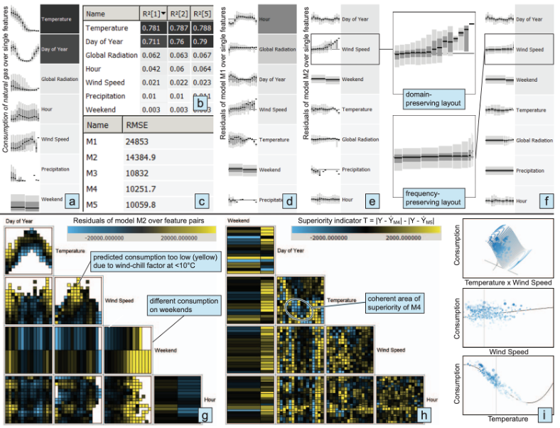 ::: ::: {.column width="45%"} **Core Visualizations:** - **Scatterplot Matrix**: Explore feature relationships and partitions - **Parallel Coordinates**: Analyze high-dimensional patterns - **Interactive Partitioning**: Split data to test model stability **Key Insights:** - Trade-off between model complexity and accuracy - Feature ranking and selection - Model validation across partitions ::: ::: ::: footer Mühlbacher, T., & Piringer, H. (2013). [A Partition-Based Framework for Building and Validating Regression Models](https://doi.org/10.1109/TVCG.2013.125). *IEEE TVCG*. **Best Paper Award, IEEE VAST 2013**. ::: ::: {.notes} This IEEE TVCG Best Paper (VAST 2013) presents an interactive system for exploring the accuracy-complexity tradeoff in linear models. The system uses scatterplot matrices to visualize relationships between features and identify potential partitions in the data. Parallel coordinates help analysts understand high-dimensional patterns and feature interactions. Users can interactively partition the data, add or remove features, and immediately see the impact on model performance metrics like R-squared and cross-validation error. This combination of visualizations helps identify the simplest model that achieves acceptable accuracy while understanding how the model performs across different data subsets. ::: ## Pros, Cons, and Limitations of Linear Models ::: {.columns} ::: {.column width="50%"} ### ✅ Pros: - **Highly interpretable**: Each coefficient has clear meaning - **Statistical guarantees**: Inference possible when assumptions hold - **Fast**: Analytical solution, no hyperparameters - **Transparent**: Easy to explain to stakeholders ::: ::: {.column width="50%"} ### ⚠️ Cons & Limitations: - **Linearity assumption**: Cannot capture non-linear relationships - **Gaussian assumption**: Features assumed to follow normal distribution - **Multicollinearity**: Correlated features break interpretation - **No interactions**: Must manually add interaction terms - **Assumption violations**: Wrong inference if residuals not normal **What if your dataset does not follow these assumptions?** ::: ::: ::: {.notes} Linear models shine when relationships are truly linear and assumptions hold (normal residuals, homoscedasticity, no multicollinearity). But real-world data often violates these assumptions - many real phenomena have non-linear relationships (e.g., diminishing returns, threshold effects) and feature interactions (e.g., temperature × humidity jointly affecting comfort). When data violates linear assumptions, we need more flexible models like GAMs. ::: ## Generalized Additive Models (GAMs) GAMs extend linear models by replacing linear terms with flexible shape functions: \begin{equation} g(\mathbb{E}[y|X]) = \beta_0 + \sum_{j=1}^{p} f_j(x_{j}) \end{equation} **Key idea:** Replace $\beta_j x_j$ (linear) with $f_j(x_j)$ (flexible smooth function) ::: {.incremental} - Each $f_j$ is learned from data (typically using splines) - Maintains additive structure → still interpretable - Can mix linear and non-linear terms ::: ::: footer Molnar, C. (2022). [*Interpretable Machine Learning*](https://christophm.github.io/interpretable-ml-book/extend-lm.html). Chapter 4.2. ::: ::: {.notes} GAMs replace linear terms with smooth functions that can capture non-linear patterns. Each feature gets its own learned shape function (often splines or smoothing functions). The model remains additive (no interactions by default) which preserves interpretability - we can visualize each function independently. The link function g allows for different target distributions (normal for regression, logistic for classification). ::: ## GAMs are Interpretable via Partial Dependence Plots (PDPs) ::: {.columns} ::: {.column width="50%"} **Linear Model:** $y = \beta_j x_j$ - Fixed slope $\beta_j$ - Constant effect across all values - Example: Each year of age adds $1,000 to salary ::: ::: {.column width="50%"} **GAM:** $y = f_j(x_j)$ - Flexible shape function - Effect varies across feature range - Example: Salary peaks at age 45-55, declines after ::: ::: **Visualization:** PDPs show $f_j(x_j)$ - the contribution of feature $x_j$ to the prediction across its range ::: {.notes} Partial Dependence Plots are what make GAMs interpretable. Instead of a single coefficient, we get a curve showing how the feature's contribution changes across its range. This reveals patterns like U-shapes (high at extremes), S-shapes (threshold effects), or plateaus (saturation). PDPs answer: "How does changing this feature affect predictions, on average?" The y-axis shows contribution relative to the mean prediction. ::: ## How GAMs Work: Splines as Building Blocks GAMs use **splines** (piecewise polynomial functions) to approximate smooth curves: ::: {.columns} ::: {.column width="50%"} **Technical approach:** - Replace feature $x_j$ with basis functions - Fit weights to these basis functions - Add penalty term for smoothness ::: ::: {.column width="50%"} **Interpretation:** - Visualize each $f_j(x_j)$ as a curve - Y-axis shows contribution to prediction - Relative to mean prediction ::: ::: ::: footer Molnar, C. (2022). [*Interpretable Machine Learning*](https://christophm.github.io/interpretable-ml-book/extend-lm.html). Chapter 4.2. ::: ::: {.notes} Under the hood, GAMs convert each feature into multiple "basis functions" (like polynomial terms or spline segments). The model learns weights for these basis functions, similar to how linear regression learns coefficients. A smoothness penalty prevents overfitting by penalizing overly wiggly curves. This is controlled by cross-validation. The result: smooth, interpretable curves showing each feature's effect. ::: ## Generalized Additive Models (GAMs): An Example \begin{equation} Wage = f(year, age, education) = b_0 + f_1(year) + f_2(age) + f_3(education) \end{equation} 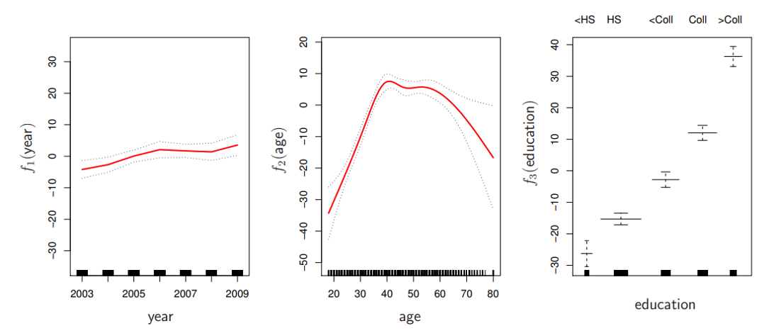 ::: {.notes} This wage prediction example shows how GAMs capture different functional forms: year has a roughly linear upward trend, age shows a non-monotonic curve peaking in mid-career years, and education shows discrete jumps between levels. Each function is learned from data while the additive structure keeps the model interpretable. ::: ## Generalized Additive Models (GAMs): Pros and Cons ::: {.columns} ::: {.column width="50%"} ### ✅ Pros: - **Non-linear flexibility**: Automatically learns smooth curves for each feature - **Better predictions**: Captures non-linear relationships without manual feature engineering - **Still interpretable**: Visualize each $f_j(x_j)$ independently - **Maintains additivity**: Easy to understand feature contributions ::: ::: {.column width="50%"} ### ⚠️ Cons: - **No interactions by default**: Must explicitly add interaction terms - **Computationally expensive**: Finding all pairwise interactions is infeasible with many features - **Harder to explain**: Shape functions less intuitive than linear coefficients - **Overfitting risk**: Requires careful smoothness tuning ::: ::: ::: {.notes} GAMs balance flexibility and interpretability nicely - more expressive than linear models but still visualizable. But the no-interaction constraint can be limiting. If temperature and humidity interact to affect outcomes (e.g., heat index), a pure GAM will miss this synergistic effect and may underfit. ::: ## Explainable Boosting Machines ::: {.columns} ::: {.column width="65%"} \begin{equation} g(\mathbb{E}[y]) = \beta_0 + \sum f_j(x_j) \end{equation} \begin{equation} g(\mathbb{E}[y]) = \beta_0 + \sum f_j(x_j) + \sum f_{ij}(x_i, x_j) \end{equation} ::: ::: {.column width="35%"} What if we have a lot of interactions? How do we choose our interactions? ::: ::: ::: {.notes} Automatically selecting which interactions to include is an active research area. EBMs use gradient boosting to greedily select the most important pairwise interactions during training. The boosting process alternates between improving main effects and interactions, naturally prioritizing the most impactful terms. ::: ## Explainable Boosting Machines ::: {style="text-align: center;"} ::: ::: {.notes} This video from Microsoft Research demonstrates the InterpretML library and EBMs in action. Watch how the system automatically discovers important feature interactions and visualizes their effects on predictions using partial dependence plots and interaction heatmaps. ::: ## Partial Dependence Plots (PDPs) ::: {.columns} ::: {.column width="60%"} **What PDPs show:** The marginal effect of a feature on the predicted outcome **Mathematical idea:** Average the model's predictions across all data points while varying one feature ::: {.incremental} - **Y-axis**: Change in prediction (relative to baseline) - **X-axis**: Feature values - **Curve shape**: Reveals linear, monotonic, or complex relationships (U-shaped in example) ::: ::: ::: {.column width="40%"} 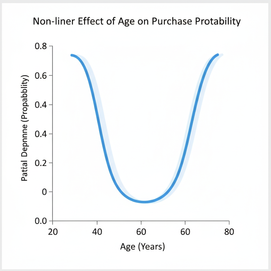{width="100%"} ::: ::: ::: footer Molnar, C. (2022). [*Interpretable Machine Learning*](https://christophm.github.io/interpretable-ml-book/pdp.html). Chapter 8.1. ::: ::: {.notes} PDPs marginalize the model output over the distribution of other features. For each value of feature X, we compute predictions for all data points with X set to that value, then average those predictions. This shows the average effect of X on predictions. The curve reveals whether the relationship is linear (straight line), monotonic (always increasing/decreasing), or more complex with peaks and valleys. ::: ## PDPs: Advantages and Limitations ::: {.columns} ::: {.column width="50%"} ### ✅ Advantages: - **Intuitive**: Easy to understand and explain - **Model-agnostic**: Works with any model - **Causal hints**: Suggests feature importance - **Shows shape**: Reveals non-linear patterns ::: ::: {.column width="50%"} ### ⚠️ Limitations: - **Independence assumption**: Assumes features are independent (often violated!) - **Averages hide details**: Misses heterogeneous effects - **Unrealistic combinations**: May average over impossible feature values - **Max 2 features**: Can't visualize high-dimensional interactions ::: ::: ::: footer Molnar, C. (2022). [*Interpretable Machine Learning*](https://christophm.github.io/interpretable-ml-book/pdp.html). Chapter 8.1. ::: ::: {.notes} The independence assumption is critical: PDPs assume you can vary one feature while holding others at their marginal distribution. But if features are correlated (e.g., house size and number of rooms), the PDP may average over unrealistic combinations. For example, it might average predictions for "1000 sq ft with 10 bedrooms" which doesn't exist in reality. ICE plots (coming next) help reveal when PDPs are misleading by showing individual trajectories instead of averages. ::: ## Visualizing EBMs (or GAMs) 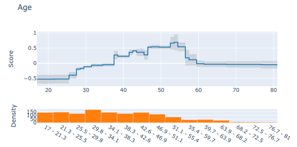 ::: {.notes} This PDP shows how predictions change as we vary one feature while marginalizing over all others. The y-axis shows the average prediction change from the baseline, making it easy to see each feature's isolated effect. The rug plot at bottom shows the distribution of actual feature values - always check this to ensure you're not extrapolating beyond the data. ::: ## Visualizing EBMs (or GAMs) 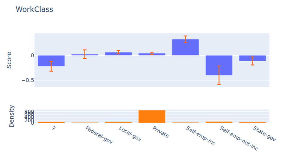 ::: {.notes} Here we see multiple partial dependence plots arranged in a dashboard layout. This allows comparing the relative importance and functional forms of different features at a glance. Features with flat lines have little effect, while steep curves indicate strong influence on predictions. ::: ## Visualizing EBMs (or GAMs)  ::: {.notes} This shows a 2D partial dependence plot for an interaction term between two features. The heatmap reveals how the two features jointly affect predictions, capturing synergistic effects that 1D plots would miss. Darker regions indicate combinations that strongly influence predictions. ::: ## Visualizing EBMs (or GAMs)  ::: {.notes} Individual Conditional Expectation (ICE) plots show how predictions change for individual instances rather than averaging across the dataset. Each line represents one data point. This reveals heterogeneity - different instances may respond differently to the same feature change, suggesting important interactions or subpopulations. ::: ## Visual Analytics (VA) Systems Using GAMs  ::: footer Hohman, F., Head, A., Caruana, R., DeLine, R., & Drucker, S. M. (2019). [Gamut: A Design Probe to Understand How Data Scientists Understand Machine Learning Models](https://doi.org/10.1145/3290605.3300809). *CHI 2019*. ::: ::: {.notes} GAMUT from Microsoft Research explores how data scientists interact with GAM visualizations through a design probe study. The system shows individual feature contributions for each observation, helping users understand both global patterns (overall feature effects) and local predictions (why this specific instance got this prediction). The research revealed that interpretability is not monolithic - data scientists have different reasons to interpret models and tailor explanations for specific audiences. ::: ## Visual Analytics (VA) Systems Using GAMs  ::: footer Drucker, S. (2020). [Data Visualization: Bridging the Gap Between Users and Information](https://www.microsoft.com/en-us/research/video/data-visualization-bridging-the-gap-between-users-and-information/). Microsoft Research Webinar. ::: ::: {.notes} This slide from Steven Drucker's Microsoft Research presentation shows a GAM visualization system with multiple coordinated views, including partial dependence plots for understanding feature effects, residual analysis for identifying model weaknesses, and instance-level explanations. Interactive brushing and linking allows users to select interesting subgroups and explore their characteristics. Drucker leads Microsoft's Visualization and Data Analysis Group (VIDA). ::: ## GAM Changer: Injecting Domain Knowledge via Interactive Editing ::: {.columns} ::: {.column width="65%"} 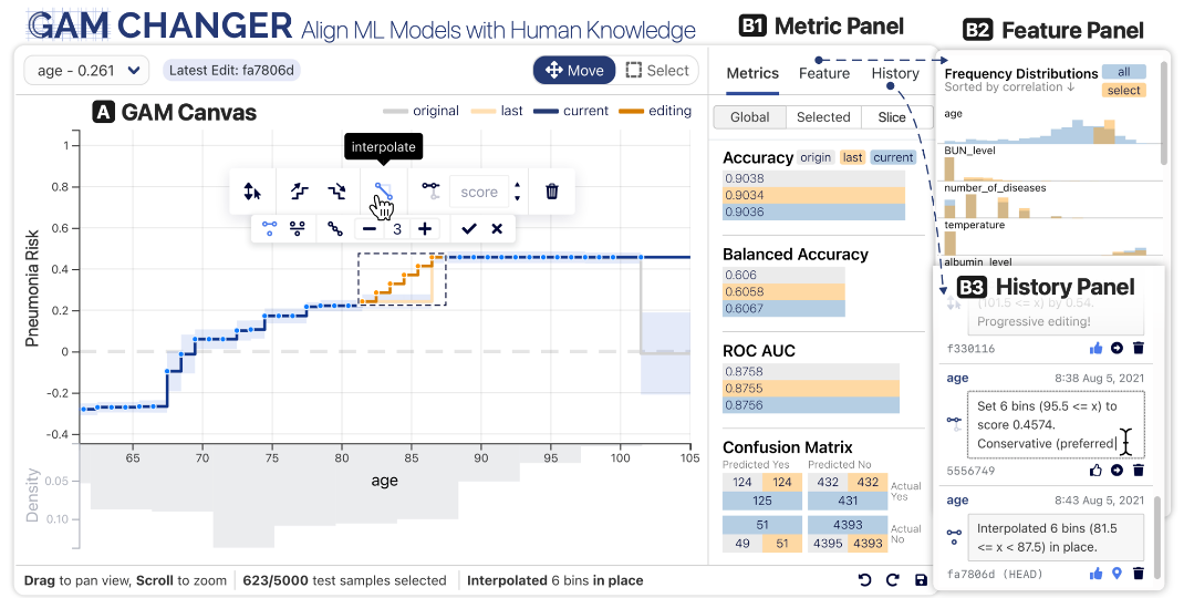 ::: ::: {.column width="35%"} **Human-in-the-Loop Features:** - **Edit shape functions** to encode domain knowledge - **Enforce monotonicity** where business logic requires - **Smooth noisy patterns** to improve generalization - **Real-time feedback** on model performance **Key Innovation:** Bridges data-driven learning with expert knowledge through interactive visualization ::: ::: ::: footer Wang, Z. J., Kale, A., Nori, H., Stella, P., Nunnally, M., Chau, D. H., ... & Caruana, R. (2021). [GAM Changer: Editing Generalized Additive Models with Interactive Visualization](https://arxiv.org/abs/2112.03245). arXiv:2112.03245. [Demo](https://interpret.ml/gam-changer/) | [Code](https://github.com/interpretml/gam-changer) ::: ::: {.notes} GAM Changer exemplifies the human-in-the-loop paradigm for model development. Users can interactively edit learned shape functions to inject domain knowledge - for example, enforcing that credit risk must monotonically increase with debt-to-income ratio, even if the data suggests otherwise due to sampling bias. Data scientists can manually adjust function shapes while seeing real-time impacts on model performance metrics. This approach is crucial when you need models that are not just accurate but also align with business logic and regulatory requirements. The tool runs locally in computational notebooks or browsers without requiring extra compute resources. ::: ## Decision Trees: How They Work ::: {.columns} ::: {.column width="50%"} Decision trees recursively split data based on feature thresholds: ::: {.incremental} - **Internal nodes**: Tests on features - **Branches**: Test outcomes (Yes/No) - **Leaf nodes**: Final predictions - **Algorithm**: CART ::: **Prediction**: Follow path from root to leaf ::: ::: {.column width="50%"} 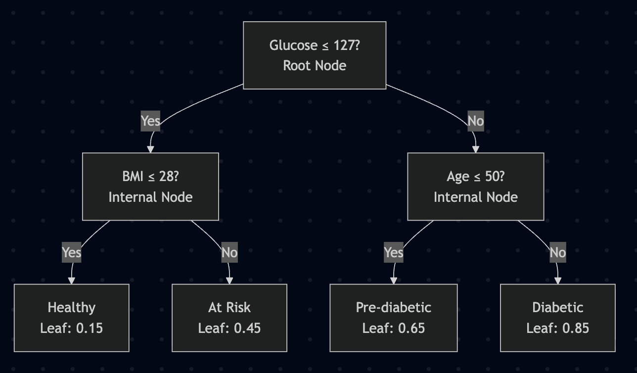{width="100%"} |Yes| B[BMI ≤ 28?
Internal Node] A -->|No| C[Age ≤ 50?
Internal Node] B -->|Yes| D[Healthy
Leaf: 0.15] B -->|No| E[At Risk
Leaf: 0.45] C -->|Yes| F[Pre-diabetic
Leaf: 0.65] C -->|No| G[Diabetic
Leaf: 0.85] style A fill:#e8f4f8,stroke:#2980b9,stroke-width:3px style B fill:#f0f8ff,stroke:#3498db,stroke-width:2px style C fill:#f0f8ff,stroke:#3498db,stroke-width:2px style D fill:#d5f4e6,stroke:#27ae60,stroke-width:2px style E fill:#fff3cd,stroke:#f39c12,stroke-width:2px style F fill:#ffd6cc,stroke:#e67e22,stroke-width:2px style G fill:#f8d7da,stroke:#e74c3c,stroke-width:2px ``` --> **Example:** 3 splits, 4 leaves, depth 2 ::: ::: ::: footer Molnar, C. (2022). [*Interpretable Machine Learning*](https://christophm.github.io/interpretable-ml-book/tree.html). Chapter 4.4. ::: ::: {.notes} Decision trees work by recursively partitioning the feature space. At each internal node, the algorithm chooses a feature and threshold that best splits the data (measured by Gini impurity for classification or variance reduction for regression). This creates a hierarchical structure where each path represents a decision rule. To make a prediction, follow the decision path from root to leaf based on the instance's feature values. ::: ## Decision Trees: Interpretation **Reading a tree**: "If feature $x_j$ is [smaller/larger] than threshold $c$ AND ... then predict $\hat{y}$" ::: {.columns} ::: {.column width="50%"} ### ✅ Strengths: - **Natural interactions**: Captures feature interactions automatically - **Visual logic**: Clear decision rules - **No preprocessing**: Works with raw features - **Human-friendly**: Mimics human reasoning ::: ::: {.column width="50%"} ### ⚠️ Limitations: - **Linear relationships**: Poor at modeling smooth trends - **High variance/instability**: Small data changes → different tree - **Depth problem**: Deep trees become uninterpretable - **Step functions**: Predictions jump at thresholds **→ This instability motivates ensemble methods** (Random Forests, Gradient Boosting) which average many trees ::: ::: **Trade-off:** Ensembles gain accuracy but **lose white-box interpretability** → Need for global surrogates (discussed later) ::: footer Molnar, C. (2022). [*Interpretable Machine Learning*](https://christophm.github.io/interpretable-ml-book/tree.html). Chapter 4.4. ::: ::: {.notes} The key limitation of decision trees is their instability (high variance) - small changes in training data can produce completely different tree structures. This motivated the development of ensemble methods like Random Forests and Gradient Boosting, which average predictions from hundreds of trees to reduce variance and improve accuracy. However, this comes at a major cost: we lose the white-box interpretability of individual trees. You can't meaningfully inspect 500 trees! This trade-off between accuracy and interpretability is why we need techniques like global surrogate models (discussed later) to explain ensemble predictions. ::: ## Tree-based Models: Example 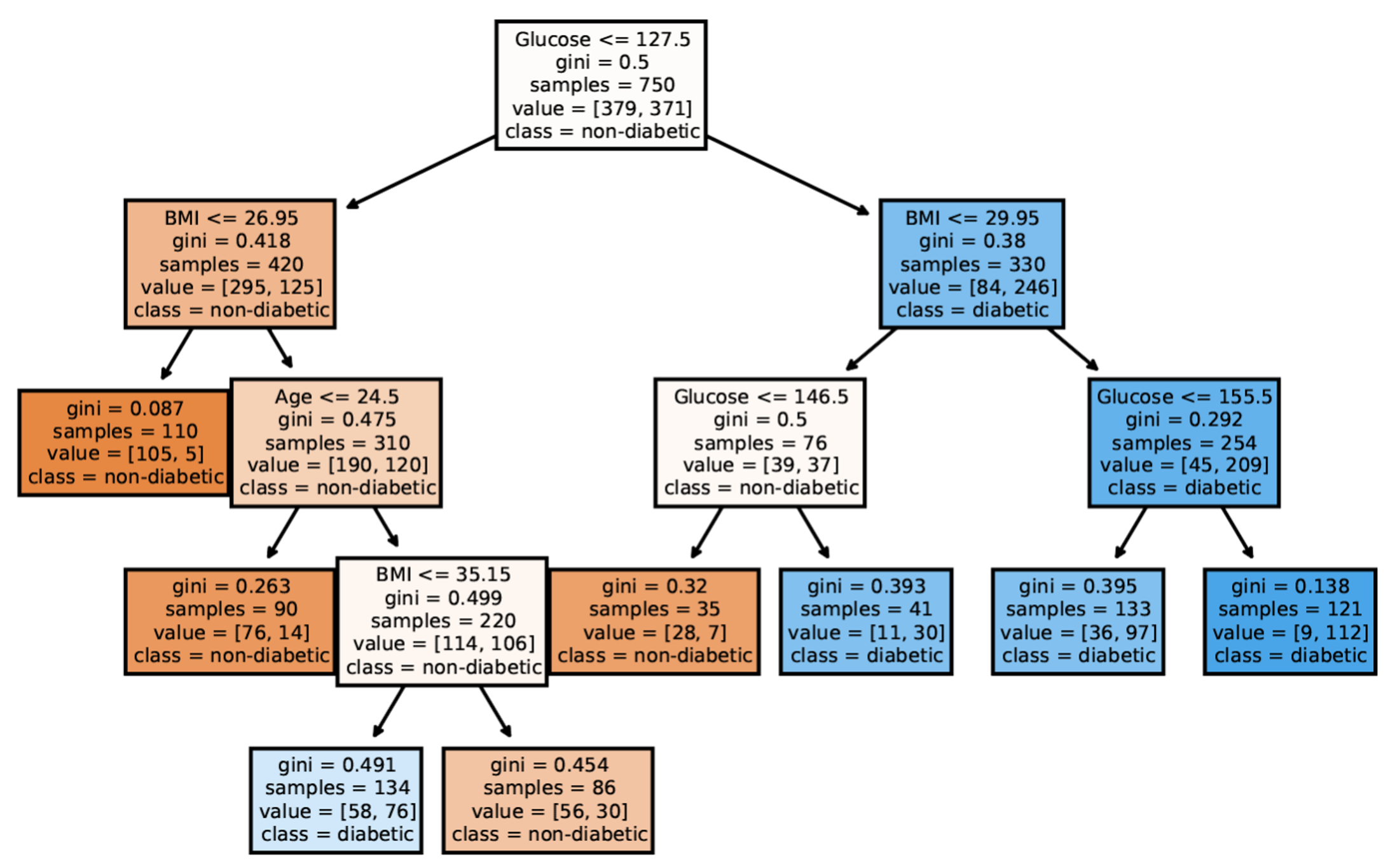 ::: {.notes} This diabetes diagnosis tree demonstrates decision tree structure in practice. Each path from root to leaf represents a decision rule with explicit conditions. The tree shows how glucose level, BMI, age, and other factors combine hierarchically to predict disease risk. Notice how the tree naturally captures interactions - the same glucose threshold might have different meanings depending on BMI. Trees are highly interpretable when shallow like this, but can become unwieldy when deep. ::: ## VA Systems Using Tree-based Models ::: {.columns} ::: {.column width="65%"} 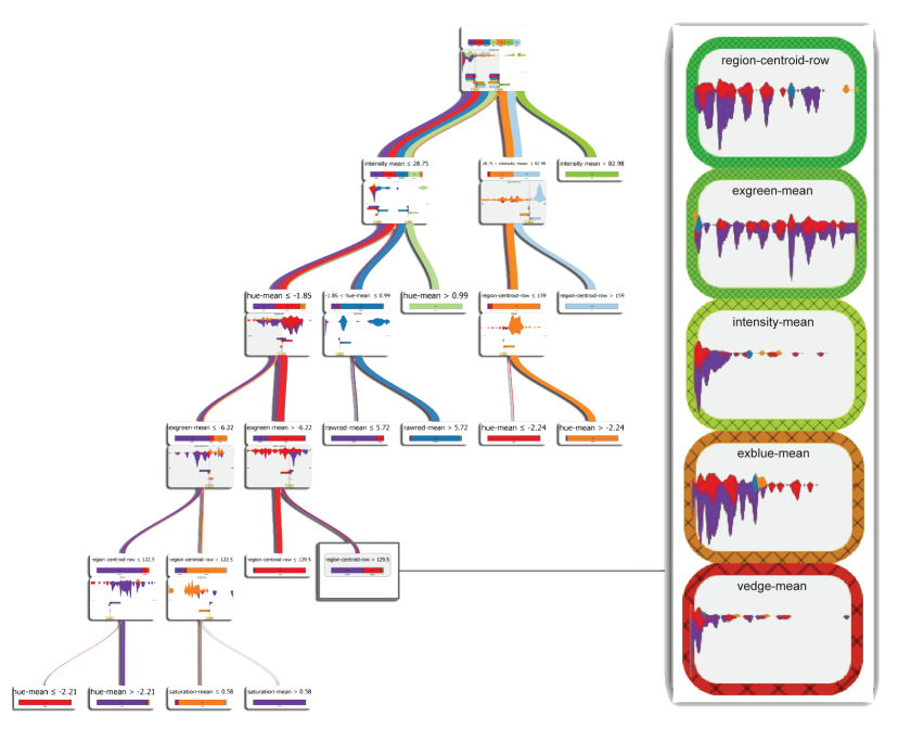 ::: ::: {.column width="35%"} It shows the flow of different class, and the class distribution along the feature values. ::: ::: ::: footer van den Elzen, S., & van Wijk, J. J. (2011). [BaobabView: Interactive Construction and Analysis of Decision Trees](https://doi.org/10.1109/VAST.2011.6102453). *IEEE VAST 2011*. ::: ::: {.notes} BaobabView (van den Elzen & van Wijk, VAST 2011) uses a custom layout optimized for classification trees. The width of edges encodes the number of instances flowing through each branch, and color shows class distribution at each node. This makes it easy to see where the model is confident vs uncertain, and which features do the most splitting work. The system allows interactive construction and analysis of decision trees. ::: ## VA Systems Using Tree-based Models 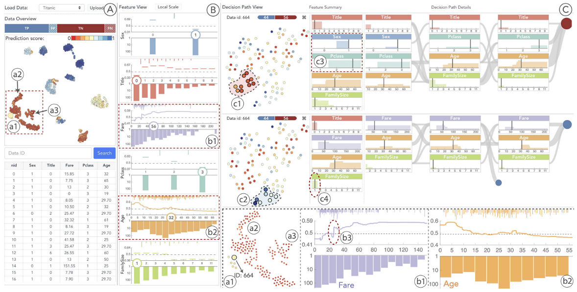 ::: footer Zhao, X., Wu, Y., Lee, D. L., & Cui, W. (2019). [iForest: Interpreting Random Forests via Visual Analytics](https://doi.org/10.1109/TVCG.2018.2864475). *IEEE TVCG*, 25(1), 407-416. ::: ::: {.notes} iForest (Zhao et al., IEEE TVCG 2019) visualizes random forest ensembles rather than individual trees. The system aggregates predictions across trees to show which regions of feature space have high consensus vs disagreement among ensemble members. Areas of disagreement may indicate decision boundaries, noisy data, or underspecified regions where the model is uncertain. This addresses the key interpretability challenge with random forests - understanding the collective behavior of many trees. ::: ## Interactive Construction and Analysis of Decision Trees ::: {.columns} ::: {.column width="50%"} 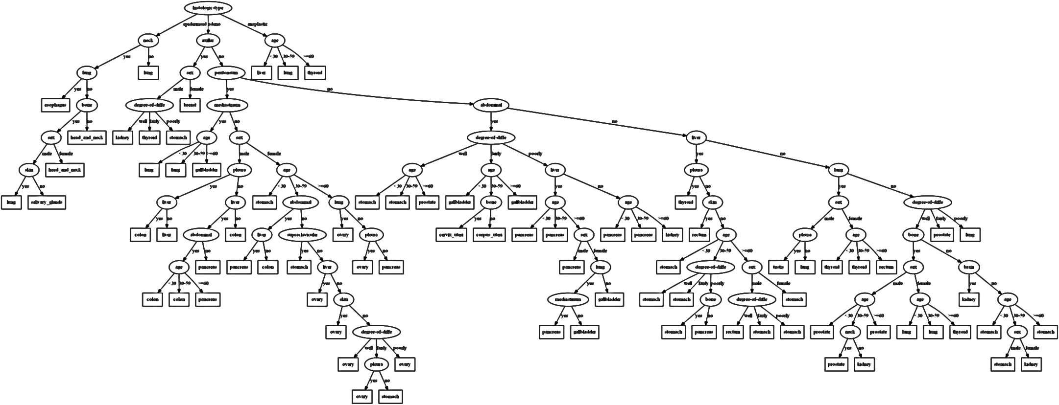 ::: ::: {.column width="50%"} - Novel node-link visualization for very large decision trees - Interactive construction: users can split nodes, prune branches - Multiple views: overview, detail, rules ::: ::: ::: {.notes} Elzen and van Wijk's VAST 2011 paper presents an interactive system for constructing and analyzing decision trees. The visualization uses a novel compact layout that can display very large trees. Users can interactively split nodes, prune branches, and explore different tree configurations. The system combines overview, detail, and rule extraction views. ::: ## Interactive Construction: Video Demonstration ::: {style="text-align: center;"} ::: ::: {.notes} This video demonstrates the interactive capabilities of the Elzen & van Wijk system. Watch how users can interactively construct decision trees, explore different splits, prune branches, and analyze the resulting tree structure. The system provides real-time feedback on tree performance as users make modifications. ::: ## Interactive Construction: Colored Flow Visualization 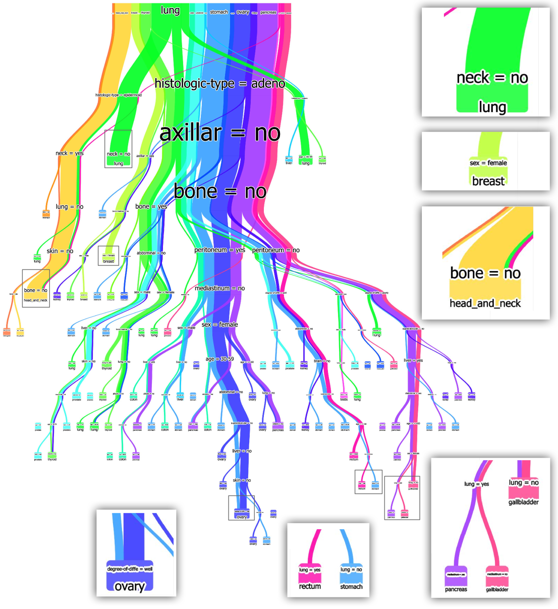 ::: {.notes} This view shows decision paths colored by class labels (e.g., neck=no, lung, breast, bone=no). The flow visualization makes it easy to trace how different classes are separated through the tree. Width encodes the number of instances following each path. This design helps identify which features are most discriminative for each class. ::: ## Interactive Construction: Rule Visualization 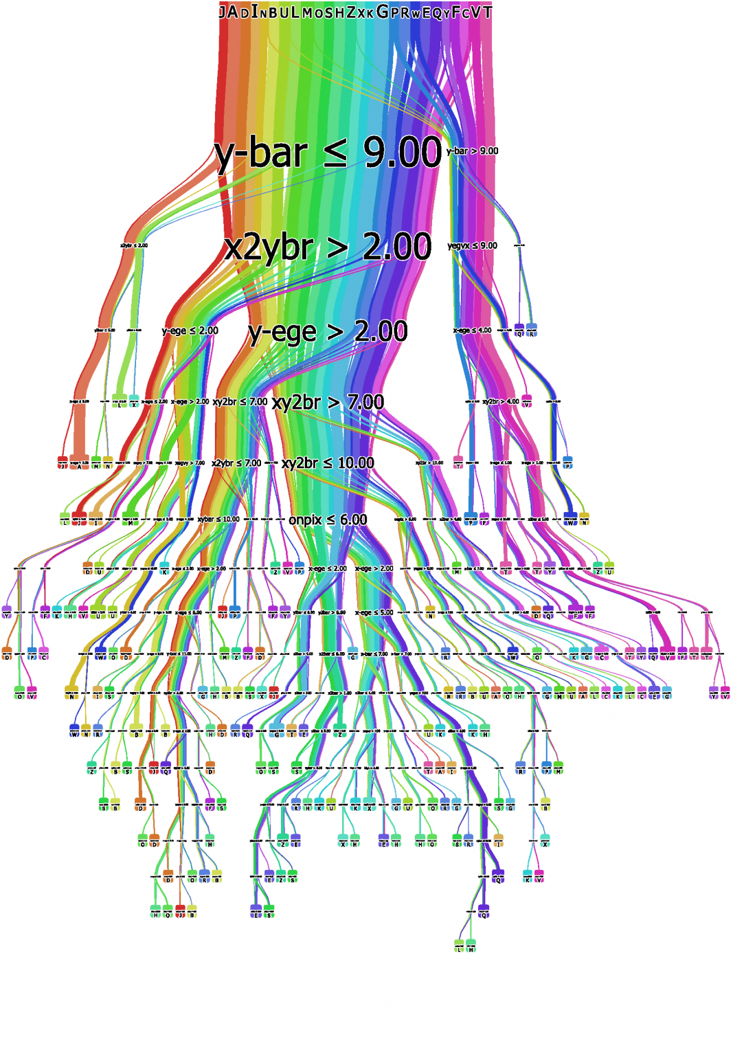 ::: {.notes} This view shows the explicit decision rules at each node (e.g., y-bar ≤ 9.00, x2ybr > 2.00). The rainbow coloring helps distinguish different paths through the tree. Users can see the complete rule set from root to any leaf, making it easy to extract interpretable decision rules from the trained tree. ::: # Decision Rules ## Decision Rules: What Are They? **Definition:** A decision rule is a simple IF-THEN statement consisting of a condition (antecedent) and a prediction (consequent). ::: {.incremental} - **Structure**: IF (condition) THEN (prediction) - **Example**: IF glucose > 120 AND age > 50 THEN diabetes_risk = high - **Natural language**: Rules mirror human decision-making processes - **Sparse representation**: Only relevant features appear in conditions - **Fast prediction**: Simple logical evaluation - **Transparent**: Each rule's logic is fully exposed - **Compliance-ready**: Rules can be directly translated into legal/regulatory documentation ::: ::: {.notes} Decision rules represent one of the most interpretable forms of machine learning models. They directly mirror human decision-making processes by explicitly stating conditions and outcomes. This makes them particularly valuable in domains where transparency and explainability are crucial, such as healthcare, finance, and legal applications. ::: ## Key Difference: Trees vs. Rule Systems ::: {.columns} ::: {.column width="50%"} **Decision Trees:** - **Mutually Exclusive**: Each instance follows exactly one path - **No conflicts**: Instance reaches exactly one leaf - **Hierarchical**: Rules are ordered by tree structure - **Example**: A patient is either "high risk" OR "low risk", never both ::: ::: {.column width="50%"} **Rule Systems:** - **Not Mutually Exclusive**: Instance can match multiple rules - **Conflict resolution needed**: Voting, priority, or confidence-based - **Flat structure**: Rules can be evaluated in any order - **Example**: A loan can trigger both "high income" AND "high debt" rules ::: ::: **Implication:** Rule systems need strategies to handle overlapping rules (majority vote, highest confidence, first match) ::: {.notes} This is a fundamental distinction often overlooked. In decision trees, the hierarchical structure guarantees mutual exclusivity - you can't be in two leaves simultaneously. Rule systems allow multiple rules to fire for the same instance, which can be more flexible but requires conflict resolution. Common strategies include: majority voting (classification), weighted average (regression), or priority ordering (first matching rule wins). ::: ## Decision Rules: Key Characteristics **Evaluation Metrics:** ::: {.incremental} - **Support**: Percentage of instances matching rule conditions - **Confidence/Accuracy**: Percentage of correct predictions when rule fires - **Coverage**: How much of the dataset is explained by the rule set ::: **Learning Approaches:** ::: {.incremental} - **OneR**: Selects single best feature, discretizes it, creates one rule per value - **Sequential Covering**: Learns rules greedily - finds best rule, removes covered instances, repeats - **Bayesian Rule Lists**: Pre-mines frequent patterns, uses Bayesian model selection for optimal ordering - **RIPPER**: Fast rule learner with pruning to prevent overfitting ::: ::: {.notes} Support measures breadth - does the rule apply to many instances? Confidence measures precision - when the rule fires, is it usually correct? Good rules balance both metrics. Very specific rules (low support) may overfit, while very general rules (high support, low confidence) may be too simplistic. Sequential covering is the classic approach: learn one rule, remove the data it covers, repeat until all data is covered. ::: ## Decision Rules: Pros and Cons ::: {.columns} ::: {.column width="50%"} ### ✅ Strengths: - **Easy to interpret**: Natural language reasoning - **Fast prediction**: Simple logical checks - **Robust**: Invariant to feature transformations - **Feature selection**: Automatically identifies relevant features - **Human-aligned**: Matches how experts explain decisions ::: ::: {.column width="50%"} ### ⚠️ Limitations: - **Regression challenges**: Works best for classification - **Feature discretization**: Continuous features need binning - **Linear relationships**: Hard to capture smooth trends - **Overfitting risk**: Complex rules may not generalize - **Rule conflicts**: Overlapping rules need resolution ::: ::: ::: footer Molnar, C. (2022). [*Interpretable Machine Learning*](https://christophm.github.io/interpretable-ml-book/rules.html). Chapter 4.7. ::: ::: {.notes} Decision rules excel when you need transparent, auditable models. They're particularly valuable in regulated industries where you must explain each decision. However, they struggle with continuous relationships - you can't easily express "price increases smoothly with size" as rules. The discretization required for continuous features can lose information and create artificial boundaries. ::: ## Decision Rules: Different Structures ::: {.columns} ::: {.column width="50%"}  Clearly see how the decision is made and which rule is more important. ::: ::: {.column width="50%"}  The final decision is made based on a voting mechanism. A recent user study shows that "if-then structure without any connecting else statements enables users to easily reason about the decision boundaries of classes." ::: ::: ::: {.notes} Rule lists have a clear priority ordering with if-then-else chains - rules are tried sequentially until one fires. Rule sets allow multiple rules to fire simultaneously and vote on the final decision. User studies show people find rule sets more intuitive because they don't require mentally tracking a cascading else chain. Each rule stands independently. ::: ## Decision Rules: Different Structures Disjunctive normal form (DNF, OR-of-ANDs) Conjunctive normal form (CNF, AND-of-ORs)  ::: {.notes} This example shows DNF (Disjunctive Normal Form) rules: each rule is a conjunction (AND) of conditions, and we predict positive if ANY rule fires (OR). DNF is more common in ML because it naturally represents disjoint decision regions in feature space. CNF would require all conditions across rules to be met simultaneously, which is less useful for classification. ::: ## Decision Rules: Visual Factors Influence Rule Understanding ::: {.columns} ::: {.column width="65%"}  ::: ::: {.column width="35%"} **Research Questions:** Can different visualizations of rules lead to different levels of understanding? What visual factors influence understanding and how do they affect rule comprehension? **Key findings:** Visual encoding choices significantly impact interpretability ::: ::: ::: footer Yuan, J., Nov, O., & Bertini, E. (2021). [*An Exploration and Validation of Visual Factors in Understanding Classification Rule Sets*](https://arxiv.org/abs/2109.09160). arXiv:2109.09160. ::: ::: {.notes} This research by Yuan et al. investigates how visual presentation affects rule comprehension. They found that factors like rule ordering, grouping, highlighting, and textual formatting all influence how quickly and accurately people understand rule-based models. Good visual design can make complex rule sets much more accessible to non-experts, while poor design obscures patterns. The study provides empirical evidence that visualization design matters as much as the underlying model for interpretability. ::: ## Evaluation of Rules Given a rule below: If $X$, then class $Y$. Support / Coverage of a rule: \begin{equation} \text{Support} = \frac{\text{number of instances that match the conditions in } X}{\text{total number of instances}} \end{equation} Confidence / Accuracy of a rule: \begin{equation} \text{Confidence} = \frac{\text{number of instances that match conditions in } X \text{ and belong to class } Y}{\text{number of instances that match conditions in } X} \end{equation} ::: {.notes} Support measures how frequently the rule applies (what fraction of data it covers). Confidence measures how accurate the rule is when it fires (what fraction of covered instances are correctly classified). Good rules balance both - high confidence but very low support means the rule is too specific. High support but low confidence means it's too general and inaccurate. ::: ## Global Surrogate Imagine that we have a black-box model (too complex to understand the internal structure), can we use white-box models to help us understand the model behavior of the black-box model?  ::: {.notes} Global surrogate models approximate a complex black-box model with an interpretable white-box model. Train a decision tree or rule set to mimic the black-box's predictions. This trades some accuracy for interpretability - you're explaining the black-box's behavior, not the underlying true relationship. Useful when you need interpretability but your best-performing model is opaque. ::: ## Global Surrogate Open the black box by understanding a "surrogate model" that approximate the behavior of the original black-box model.  ::: {.notes} The surrogate training process: feed data through the black-box to get predictions, then train an interpretable model (decision tree, linear model, rules) to predict what the black-box would predict. The surrogate's feature importances and structure reveal what the black-box learned. Check surrogate fidelity - how well does it match the black-box predictions? ::: ## The Fidelity-Interpretability Trade-off **The Fidelity-Interpretability Trade-off:** A fundamental challenge in XAI where increasing model interpretability often decreases fidelity to the original model's behavior **What you want:** {width=540px} Simple, interpretable surrogate with high fidelity to the black-box model **What you get:** {width=540px} Either low fidelity (simple but inaccurate) or low interpretability (accurate but complex) ::: {.notes} This is the Fidelity-Interpretability Trade-off, a foundational problem in Explainable AI (XAI). You want a simple, interpretable surrogate that's also highly faithful to the black-box model's decisions. But there's an inherent tension: simple surrogates miss important patterns (low fidelity), while high-fidelity surrogates become too complex to interpret. This trade-off appears throughout XAI - in global surrogates, local explanations (LIME/SHAP), and even in choosing between white-box and black-box models initially. Understanding this trade-off is crucial for setting realistic expectations about what explanations can achieve. ::: ## VA System for Rule List  ::: footer Ming, Y., Qu, H., & Bertini, E. (2019). [RuleMatrix: Visualizing and Understanding Classifiers with Rules](https://doi.org/10.1109/TVCG.2018.2864812). *IEEE TVCG*, 25(1), 342-352. ::: ::: {.notes} RuleMatrix visualizes rule lists using a matrix layout where rows are rules and columns are features. Cell color/intensity shows feature values in each rule's conditions. This compact representation lets you quickly scan for redundant rules, identify which features are most commonly used, and spot patterns across the rule set. Interactive features support rule refinement and editing. ::: ## VA Systems for Rules in Random Forest 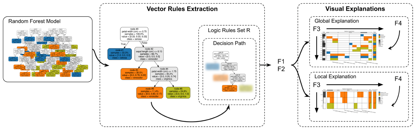 ::: footer Popolin Neto, M., & Paulovich, F. V. (2020). [Explainable Matrix -- Visualization for Global and Local Interpretability of Random Forest Classification Ensembles](https://doi.org/10.1109/TVCG.2020.3030354). *IEEE TVCG*, 27(2), 1427-1437. ::: ::: {.notes} Explainable Matrix extends rule visualization to random forest ensembles. Each tree generates rules, and the system aggregates and visualizes rule consensus across the forest. Users can see which rules appear consistently vs which are unique to specific trees. This helps understand ensemble behavior and identify stable patterns that the forest relies on. ::: ## Other white-box models? - Naive Bayes - K-nearest neighbors - etc. ::: {.notes} Beyond the models we've covered, other naturally interpretable models include: Naive Bayes (shows probability contributions from each feature via Bayes rule), K-Nearest Neighbors (predictions explained by showing similar training examples), and Logistic Regression (similar to linear regression but for classification). Each provides different forms of interpretability suited to different explanation needs. ::: ## Outline - Model Interpretation and Explanation - White-box Approaches and Visualizations - Related Research in VIS & AI ## Manipulating and Measuring Model Interpretability 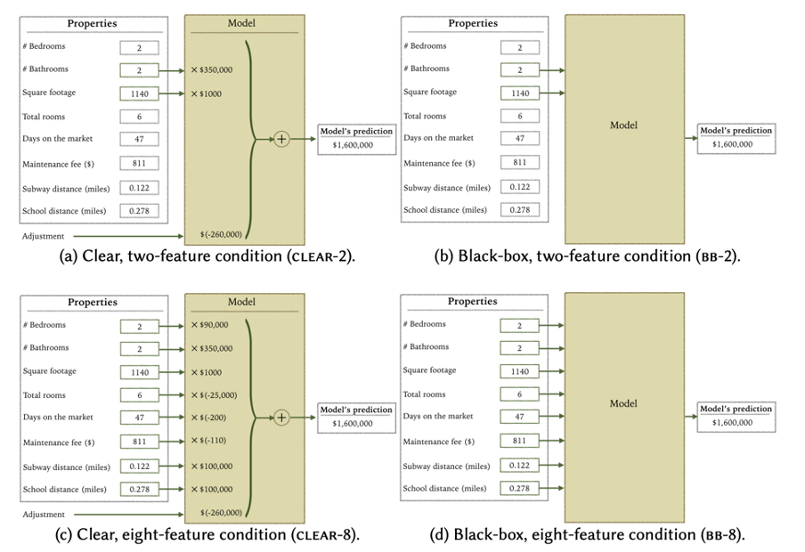 ::: footer Poursabzi-Sangdeh, F., Goldstein, D. G., Hofman, J. M., Vaughan, J. W., & Wallach, H. (2021). [Manipulating and Measuring Model Interpretability](https://arxiv.org/abs/1802.07810). *CHI 2021*. ::: ::: {.notes} This paper asks fundamental questions: Can we quantitatively measure interpretability? Can we manipulate model structure to increase interpretability while maintaining performance? The authors propose metrics for tree complexity, sparsity, and other interpretability factors. This work is important because it moves interpretability from a vague concept to something measurable and optimizable. ::: ## Stop explaining black box machine learning models for high stakes decisions 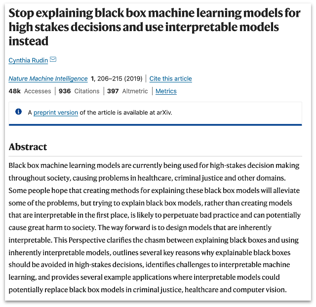 ::: footer Rudin, C. (2019). [Stop explaining black box machine learning models for high stakes decisions and use interpretable models instead](https://doi.org/10.1038/s42256-019-0048-x). *Nature Machine Intelligence*, 1(5), 206-215. ::: ::: {.notes} Cynthia Rudin's influential paper argues that for high-stakes decisions (healthcare, criminal justice, lending), we should use inherently interpretable models rather than explaining black-boxes post-hoc. Post-hoc explanations can be misleading, incomplete, or unfaithful to the model. Instead, invest effort in building accurate interpretable models from the start. This sparked important debates about the interpretability-accuracy tradeoff. ::: ## Slice Finder: Automated Data Slicing for Model Validation ::: footer Chung, Y., Kraska, T., Polyzotis, N., Tae, K. H., & Whang, S. E. (2019). [Slice Finder: Automated Data Slicing for Model Validation](https://doi.org/10.1109/ICDE.2019.00094). *IEEE ICDE 2019*, 1028-1039. ::: ::: {.columns} ::: {.column width="50%"} 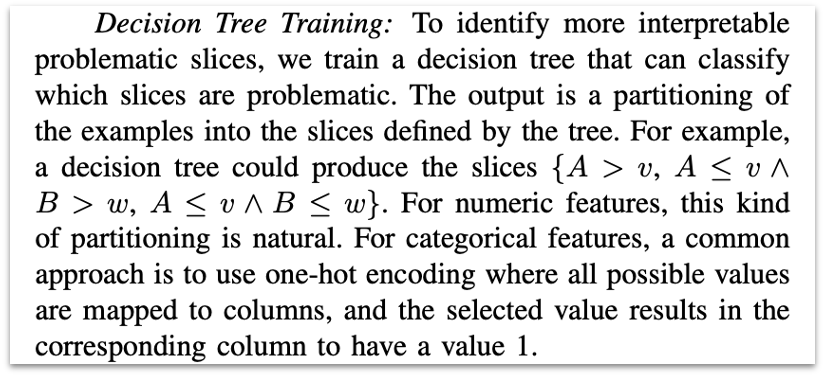 ::: :::{.column width="50%"} How about we use whether the model prediction is wrong or not to train a "surrogate tree"? ::: ::: ::: {.notes} Slice Finder uses a clever approach: train a decision tree to predict where your model makes errors. The tree splits identify data slices where performance degrades. This automates the manual process of searching for problematic subgroups. The resulting tree provides an interpretable description of failure modes - "the model struggles when age > 65 AND income < 30k". ::: ## Toolkits InterpretML: https://github.com/interpretml/interpret ::: {.notes} InterpretML is Microsoft's open-source library for interpretable machine learning. It implements GAMs, Explainable Boosting Machines (EBMs), and various explanation techniques. The library includes both glass-box models (inherently interpretable) and black-box explanation methods (LIME, SHAP). It provides unified APIs and visualization tools, making it easy to compare different interpretability approaches. Highly recommended for practical work. ::: ## Practice 1 Notebook: https://colab.research.google.com/drive/1nKE6WIApebHi67yfhH6k5mZN86evLZOM?usp=sharing Some other libraries for PDP visualization: https://scikit-learn.org/stable/modules/partial_dependence.html https://interpret.ml/docs/pdp.html ::: {.notes} This hands-on exercise walks through training GAMs with Python's interpret library and creating partial dependence visualizations. You'll explore how to identify non-linear patterns, detect feature interactions, and interpret model behavior through visualizations. Try comparing linear regression vs GAM on the same dataset. ::: ## Practice 2 Notebook: https://colab.research.google.com/drive/12LV2Z_1BbP3efACYp2QxzsPaOrIn8a8l?usp=sharing ::: {.notes} This hands-on exercise covers decision tree training, visualization, and rule extraction with sklearn. You'll experiment with tree depth, pruning strategies, and extracting interpretable rules from trained trees. Try comparing different tree visualization libraries and see how tree structure affects interpretability and performance. :::